Chapter 17. Decision Trees
A tree is an incomprehensible mystery.
Jim Woodring
DataSciencester’s VP of Talent has interviewed a number of job candidates from the site, with varying degrees of success. He’s collected a dataset consisting of several (qualitative) attributes of each candidate, as well as whether that candidate interviewed well or poorly. Could you, he asks, use this data to build a model identifying which candidates will interview well, so that he doesn’t have to waste time conducting interviews?
This seems like a good fit for a decision tree, another predictive modeling tool in the data scientist’s kit.
What Is a Decision Tree?
A decision tree uses a tree structure to represent a number of possible decision paths and an outcome for each path.
If you have ever played the game Twenty Questions, then you are familiar with decision trees. For example:
-
“I am thinking of an animal.”
-
“Does it have more than five legs?”
-
“No.”
-
“Is it delicious?”
-
“No.”
-
“Does it appear on the back of the Australian five-cent coin?”
-
“Yes.”
-
“Is it an echidna?”
-
“Yes, it is!”
This corresponds to the path:
“Not more than 5 legs” → “Not delicious” → “On the 5-cent coin” → “Echidna!”
in an idiosyncratic (and not very comprehensive) “guess the animal” decision tree (Figure 17-1).
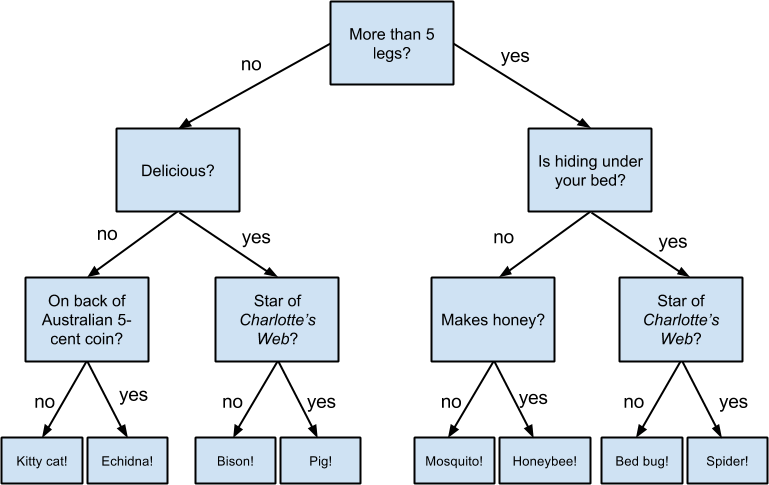
Figure 17-1. A “guess the animal” decision tree
Decision trees have a lot to recommend them. They’re very easy to understand and interpret, and the process by which they reach a prediction is completely transparent. Unlike the other models we’ve looked at so far, decision trees can easily handle a mix of numeric (e.g., number of legs) and categorical (e.g., delicious/not delicious) attributes and can even classify data for which attributes are missing.
At the same time, finding an “optimal” decision tree for a set of training data is computationally a very hard problem. (We will get around this by trying to build a good-enough tree rather than an optimal one, although for large datasets this can still be a lot of work.) More important, it is very easy (and very bad) to build decision trees that are overfitted to the training data, and that don’t generalize well to unseen data. We’ll look at ways to address this.
Most people divide decision trees into classification trees (which produce categorical outputs) and regression trees (which produce numeric outputs). In this chapter, we’ll focus on classification trees, and we’ll work through the ID3 algorithm for learning a decision tree from a set of labeled data, which should help us understand how decision trees actually work. To make things simple, we’ll restrict ourselves to problems with binary outputs like “Should I hire this candidate?” or “Should I show this website visitor advertisement A or advertisement B?” or “Will eating this food I found in the office fridge make me sick?”
Entropy
In order to build a decision tree, we will need to decide what questions to ask and in what order. At each stage of the tree there are some possibilities we’ve eliminated and some that we haven’t. After learning that an animal doesn’t have more than five legs, we’ve eliminated the possibility that it’s a grasshopper. We haven’t eliminated the possibility that it’s a duck. Each possible question partitions the remaining possibilities according to its answer.
Ideally, we’d like to choose questions whose answers give a lot of information about what our tree should predict. If there’s a single yes/no question for which “yes” answers always correspond to True outputs and “no” answers to False outputs (or vice versa), this would be an awesome question to pick. Conversely, a yes/no question for which neither answer gives you much new information about what the prediction should be is probably not a good choice.
We capture this notion of “how much information” with entropy. You have probably heard this term used to mean disorder. We use it to represent the uncertainty associated with data.
Imagine that we have a set S of data, each member of which is labeled as belonging to one of a finite number of classes . If all the data points belong to a single class, then there is no real uncertainty, which means we’d like there to be low entropy. If the data points are evenly spread across the classes, there is a lot of uncertainty and we’d like there to be high entropy.
In math terms, if is the proportion of data labeled as class , we define the entropy as:
with the (standard) convention that .
Without worrying too much about the grisly details, each term is non-negative and is close to 0 precisely when is either close to 0 or close to 1 (Figure 17-2).

Figure 17-2. A graph of -p log p
This means the entropy will be small when every is close to 0 or 1 (i.e., when most of the data is in a single class), and it will be larger when many of the ’s are not close to 0 (i.e., when the data is spread across multiple classes). This is exactly the behavior we desire.
It is easy enough to roll all of this into a function:
fromtypingimportListimportmathdefentropy(class_probabilities:List[float])->float:"""Given a list of class probabilities, compute the entropy"""returnsum(-p*math.log(p,2)forpinclass_probabilitiesifp>0)# ignore zero probabilitiesassertentropy([1.0])==0assertentropy([0.5,0.5])==1assert0.81<entropy([0.25,0.75])<0.82
Our data will consist of pairs (input, label), which means that we’ll need to compute the class probabilities ourselves. Notice that we don’t actually care which label is associated with each probability, only what the probabilities are:
fromtypingimportAnyfromcollectionsimportCounterdefclass_probabilities(labels:List[Any])->List[float]:total_count=len(labels)return[count/total_countforcountinCounter(labels).values()]defdata_entropy(labels:List[Any])->float:returnentropy(class_probabilities(labels))assertdata_entropy(['a'])==0assertdata_entropy([True,False])==1assertdata_entropy([3,4,4,4])==entropy([0.25,0.75])
The Entropy of a Partition
What we’ve done so far is compute the entropy (think “uncertainty”) of a single set of labeled data. Now, each stage of a decision tree involves asking a question whose answer partitions data into one or (hopefully) more subsets. For instance, our “does it have more than five legs?” question partitions animals into those that have more than five legs (e.g., spiders) and those that don’t (e.g., echidnas).
Correspondingly, we’d like some notion of the entropy that results from partitioning a set of data in a certain way. We want a partition to have low entropy if it splits the data into subsets that themselves have low entropy (i.e., are highly certain), and high entropy if it contains subsets that (are large and) have high entropy (i.e., are highly uncertain).
For example, my “Australian five-cent coin” question was pretty dumb (albeit pretty lucky!), as it partitioned the remaining animals at that point into = {echidna} and = {everything else}, where is both large and high-entropy. ( has no entropy, but it represents a small fraction of the remaining “classes.”)
Mathematically, if we partition our data S into subsets containing proportions of the data, then we compute the entropy of the partition as a weighted sum:
which we can implement as:
defpartition_entropy(subsets:List[List[Any]])->float:"""Returns the entropy from this partition of data into subsets"""total_count=sum(len(subset)forsubsetinsubsets)returnsum(data_entropy(subset)*len(subset)/total_countforsubsetinsubsets)
Note
One problem with this approach is that partitioning by an attribute with many different values will result in a very low entropy due to overfitting. For example, imagine you work for a bank and are trying to build a decision tree to predict which of your customers are likely to default on their mortgages, using some historical data as your training set. Imagine further that the dataset contains each customer’s Social Security number. Partitioning on SSN will produce one-person subsets, each of which necessarily has zero entropy. But a model that relies on SSN is certain not to generalize beyond the training set. For this reason, you should probably try to avoid (or bucket, if appropriate) attributes with large numbers of possible values when creating decision trees.
Creating a Decision Tree
The VP provides you with the interviewee data, consisting of (per your specification)
a NamedTuple of the relevant attributes for each candidate—her level, her preferred language, whether she is active on Twitter, whether she has a PhD, and whether she interviewed well:
fromtypingimportNamedTuple,OptionalclassCandidate(NamedTuple):level:strlang:strtweets:boolphd:booldid_well:Optional[bool]=None# allow unlabeled data# level lang tweets phd did_wellinputs=[Candidate('Senior','Java',False,False,False),Candidate('Senior','Java',False,True,False),Candidate('Mid','Python',False,False,True),Candidate('Junior','Python',False,False,True),Candidate('Junior','R',True,False,True),Candidate('Junior','R',True,True,False),Candidate('Mid','R',True,True,True),Candidate('Senior','Python',False,False,False),Candidate('Senior','R',True,False,True),Candidate('Junior','Python',True,False,True),Candidate('Senior','Python',True,True,True),Candidate('Mid','Python',False,True,True),Candidate('Mid','Java',True,False,True),Candidate('Junior','Python',False,True,False)]
Our tree will consist of decision nodes (which ask a question and direct us differently depending on the answer) and leaf nodes (which give us a prediction). We will build it using the relatively simple ID3 algorithm, which operates in the following manner. Let’s say we’re given some labeled data, and a list of attributes to consider branching on:
-
If the data all have the same label, create a leaf node that predicts that label and then stop.
-
If the list of attributes is empty (i.e., there are no more possible questions to ask), create a leaf node that predicts the most common label and then stop.
-
Otherwise, try partitioning the data by each of the attributes.
-
Choose the partition with the lowest partition entropy.
-
Add a decision node based on the chosen attribute.
-
Recur on each partitioned subset using the remaining attributes.
This is what’s known as a “greedy” algorithm because, at each step, it chooses the most immediately best option. Given a dataset, there may be a better tree with a worse-looking first move. If so, this algorithm won’t find it. Nonetheless, it is relatively easy to understand and implement, which makes it a good place to begin exploring decision trees.
Let’s manually go through these steps on the interviewee dataset. The dataset has both True and False labels, and we have four attributes we can split on. So our first step will be to find the partition with the least entropy. We’ll start by writing a function that does the partitioning:
fromtypingimportDict,TypeVarfromcollectionsimportdefaultdictT=TypeVar('T')# generic type for inputsdefpartition_by(inputs:List[T],attribute:str)->Dict[Any,List[T]]:"""Partition the inputs into lists based on the specified attribute."""partitions:Dict[Any,List[T]]=defaultdict(list)forinputininputs:key=getattr(input,attribute)# value of the specified attributepartitions[key].append(input)# add input to the correct partitionreturnpartitions
and one that uses it to compute entropy:
defpartition_entropy_by(inputs:List[Any],attribute:str,label_attribute:str)->float:"""Compute the entropy corresponding to the given partition"""# partitions consist of our inputspartitions=partition_by(inputs,attribute)# but partition_entropy needs just the class labelslabels=[[getattr(input,label_attribute)forinputinpartition]forpartitioninpartitions.values()]returnpartition_entropy(labels)
Then we just need to find the minimum-entropy partition for the whole dataset:
forkeyin['level','lang','tweets','phd']:(key,partition_entropy_by(inputs,key,'did_well'))assert0.69<partition_entropy_by(inputs,'level','did_well')<0.70assert0.86<partition_entropy_by(inputs,'lang','did_well')<0.87assert0.78<partition_entropy_by(inputs,'tweets','did_well')<0.79assert0.89<partition_entropy_by(inputs,'phd','did_well')<0.90
The lowest entropy comes from splitting on level, so we’ll need to make a subtree for each possible level value. Every Mid candidate is labeled True, which means that the Mid subtree is simply a leaf node predicting True. For Senior candidates, we have a mix of Trues and Falses, so we need to split again:
senior_inputs=[inputforinputininputsifinput.level=='Senior']assert0.4==partition_entropy_by(senior_inputs,'lang','did_well')assert0.0==partition_entropy_by(senior_inputs,'tweets','did_well')assert0.95<partition_entropy_by(senior_inputs,'phd','did_well')<0.96
This shows us that our next split should be on tweets, which results in a zero-entropy partition. For these Senior-level candidates, “yes” tweets always result in True while “no” tweets always result in False.
Finally, if we do the same thing for the Junior candidates, we end up splitting on phd, after which we find that no PhD always results in True and PhD always results in False.
Figure 17-3 shows the complete decision tree.
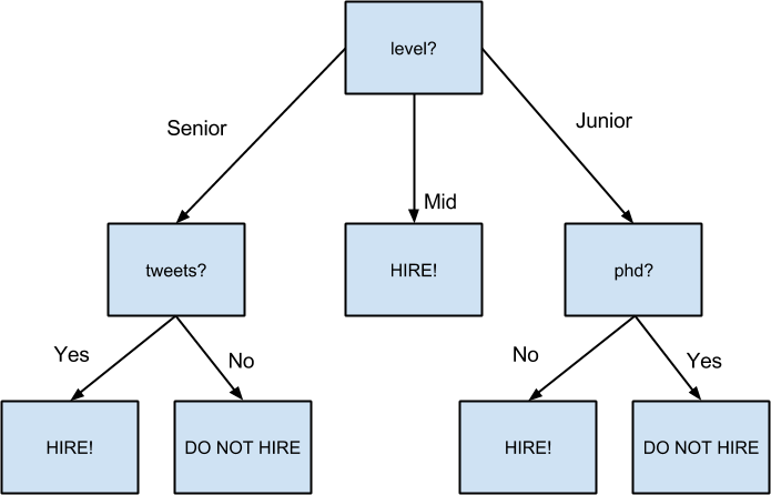
Figure 17-3. The decision tree for hiring
Putting It All Together
Now that we’ve seen how the algorithm works, we would like to implement it more generally. This means we need to decide how we want to represent trees. We’ll use pretty much the most lightweight representation possible. We define a tree to be either:
-
a
Leaf(that predicts a single value), or -
a
Split(containing an attribute to split on, subtrees for specific values of that attribute, and possibly a default value to use if we see an unknown value).fromtypingimportNamedTuple,Union,AnyclassLeaf(NamedTuple):value:AnyclassSplit(NamedTuple):attribute:strsubtrees:dictdefault_value:Any=NoneDecisionTree=Union[Leaf,Split]
With this representation, our hiring tree would look like:
hiring_tree=Split('level',{# first, consider "level"'Junior':Split('phd',{# if level is "Junior", next look at "phd"False:Leaf(True),# if "phd" is False, predict TrueTrue:Leaf(False)# if "phd" is True, predict False}),'Mid':Leaf(True),# if level is "Mid", just predict True'Senior':Split('tweets',{# if level is "Senior", look at "tweets"False:Leaf(False),# if "tweets" is False, predict FalseTrue:Leaf(True)# if "tweets" is True, predict True})})
There’s still the question of what to do if we encounter an unexpected (or missing) attribute value. What should our hiring tree do if it encounters a candidate whose level is Intern? We’ll handle this case by populating the default_value attribute with the most common label.
Given such a representation, we can classify an input with:
defclassify(tree:DecisionTree,input:Any)->Any:"""classify the input using the given decision tree"""# If this is a leaf node, return its valueifisinstance(tree,Leaf):returntree.value# Otherwise this tree consists of an attribute to split on# and a dictionary whose keys are values of that attribute# and whose values are subtrees to consider nextsubtree_key=getattr(input,tree.attribute)ifsubtree_keynotintree.subtrees:# If no subtree for key,returntree.default_value# return the default value.subtree=tree.subtrees[subtree_key]# Choose the appropriate subtreereturnclassify(subtree,input)# and use it to classify the input.
All that’s left is to build the tree representation from our training data:
defbuild_tree_id3(inputs:List[Any],split_attributes:List[str],target_attribute:str)->DecisionTree:# Count target labelslabel_counts=Counter(getattr(input,target_attribute)forinputininputs)most_common_label=label_counts.most_common(1)[0][0]# If there's a unique label, predict itiflen(label_counts)==1:returnLeaf(most_common_label)# If no split attributes left, return the majority labelifnotsplit_attributes:returnLeaf(most_common_label)# Otherwise split by the best attributedefsplit_entropy(attribute:str)->float:"""Helper function for finding the best attribute"""returnpartition_entropy_by(inputs,attribute,target_attribute)best_attribute=min(split_attributes,key=split_entropy)partitions=partition_by(inputs,best_attribute)new_attributes=[aforainsplit_attributesifa!=best_attribute]# Recursively build the subtreessubtrees={attribute_value:build_tree_id3(subset,new_attributes,target_attribute)forattribute_value,subsetinpartitions.items()}returnSplit(best_attribute,subtrees,default_value=most_common_label)
In the tree we built, every leaf consisted entirely of True inputs or entirely of False inputs. This means that the tree predicts perfectly on the training dataset. But we can also apply it to new data that wasn’t in the training set:
tree=build_tree_id3(inputs,['level','lang','tweets','phd'],'did_well')# Should predict Trueassertclassify(tree,Candidate("Junior","Java",True,False))# Should predict Falseassertnotclassify(tree,Candidate("Junior","Java",True,True))
And also to data with unexpected values:
# Should predict Trueassertclassify(tree,Candidate("Intern","Java",True,True))
Note
Since our goal was mainly to demonstrate how to build a tree, we built the tree using the entire dataset. As always, if we were really trying to create a good model for something, we would have collected more data and split it into train/validation/test subsets.
Random Forests
Given how closely decision trees can fit themselves to their training data, it’s not surprising that they have a tendency to overfit. One way of avoiding this is a technique called random forests, in which we build multiple decision trees and combine their outputs. If they’re classification trees, we might let them vote; if they’re regression trees, we might average their predictions.
Our tree-building process was deterministic, so how do we get random trees?
One piece involves bootstrapping data (recall “Digression: The Bootstrap”). Rather than training each tree on all the inputs in the training set, we train each tree on the result of bootstrap_sample(inputs). Since each tree is built using different data, each tree will be different from every other tree. (A side benefit is that it’s totally fair to use the nonsampled data to test each tree, which means you can get away with using all of your data as the training set if you are clever in how you measure performance.) This technique is known as bootstrap aggregating or bagging.
A second source of randomness involves changing the way we choose the best_attribute to split on.
Rather than looking at all the remaining attributes, we first choose a random subset of them
and then split on whichever of those is best:
# if there are already few enough split candidates, look at all of themiflen(split_candidates)<=self.num_split_candidates:sampled_split_candidates=split_candidates# otherwise pick a random sampleelse:sampled_split_candidates=random.sample(split_candidates,self.num_split_candidates)# now choose the best attribute only from those candidatesbest_attribute=min(sampled_split_candidates,key=split_entropy)partitions=partition_by(inputs,best_attribute)
This is an example of a broader technique called ensemble learning in which we combine several weak learners (typically high-bias, low-variance models) in order to produce an overall strong model.
For Further Exploration
-
scikit-learn has many decision tree models. It also has an
ensemblemodule that includes aRandomForestClassifieras well as other ensemble methods. -
XGBoost is a library for training gradient boosted decision trees that tends to win a lot of Kaggle-style machine learning competitions.
-
We’ve barely scratched the surface of decision trees and their algorithms. Wikipedia is a good starting point for broader exploration.