Chapter 22. Network Analysis

Your connections to all the things around you literally define who you are.

Aaron O’Connell

Many interesting data problems can be fruitfully thought of in terms of networks, consisting of nodes of some type and the edges that join them.

For instance, your Facebook friends form the nodes of a network whose edges are friendship relations. A less obvious example is the World Wide Web itself, with each web page a node and each hyperlink from one page to another an edge.

Facebook friendship is mutual—if I am Facebook friends with you, then necessarily you are friends with me. In this case, we say that the edges are undirected. Hyperlinks are not—my website links to whitehouse.gov, but (for reasons inexplicable to me) whitehouse.gov refuses to link to my website. We call these types of edges directed. We’ll look at both kinds of networks.

Betweenness Centrality

In Chapter 1, we computed the key connectors in the DataSciencester network by counting the number of friends each user had. Now we have enough machinery to take a look at other approaches. We will use the same network, but now we’ll use NamedTuples for the data.

Recall that the network (Figure 22-1) comprised users:

from typing import NamedTuple

class User(NamedTuple):
    id: int
    name: str

users = [User(0, "Hero"), User(1, "Dunn"), User(2, "Sue"), User(3, "Chi"),
         User(4, "Thor"), User(5, "Clive"), User(6, "Hicks"),
         User(7, "Devin"), User(8, "Kate"), User(9, "Klein")]

and friendships:

friend_pairs = [(0, 1), (0, 2), (1, 2), (1, 3), (2, 3), (3, 4),
                (4, 5), (5, 6), (5, 7), (6, 8), (7, 8), (8, 9)]

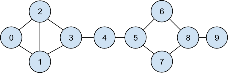
Figure 22-1. The DataSciencester network

The friendships will be easier to work with as a dict:

from typing import Dict, List

# type alias for keeping track of Friendships
Friendships = Dict[int, List[int]]

friendships: Friendships = {user.id: [] for user in users}

for i, j in friend_pairs:
    friendships[i].append(j)
    friendships[j].append(i)

assert friendships[4] == [3, 5]
assert friendships[8] == [6, 7, 9]

When we left off we were dissatisfied with our notion of degree centrality, which didn’t really agree with our intuition about who the key connectors of the network were.

An alternative metric is betweenness centrality, which identifies people who frequently are on the shortest paths between pairs of other people. In particular, the betweenness centrality of node i is computed by adding up, for every other pair of nodes j and k, the proportion of shortest paths between node j and node k that pass through i.

That is, to figure out Thor’s betweenness centrality, we’ll need to compute all the shortest paths between all pairs of people who aren’t Thor. And then we’ll need to count how many of those shortest paths pass through Thor. For instance, the only shortest path between Chi (id 3) and Clive (id 5) passes through Thor, while neither of the two shortest paths between Hero (id 0) and Chi (id 3) does.

So, as a first step, we’ll need to figure out the shortest paths between all pairs of people. There are some pretty sophisticated algorithms for doing so efficiently, but (as is almost always the case) we will use a less efficient, easier-to-understand algorithm.

This algorithm (an implementation of breadth-first search) is one of the more complicated ones in the book, so let’s talk through it carefully:

1. Our goal is a function that takes a from_user and finds all shortest paths to every other user.

2. We’ll represent a path as a list of user IDs. Since every path starts at from_user, we won’t include her ID in the list. This means that the length of the list representing the path will be the length of the path itself.

3. We’ll maintain a dictionary called shortest_paths_to where the keys are user IDs and the values are lists of paths that end at the user with the specified ID. If there is a unique shortest path, the list will just contain that one path. If there are multiple shortest paths, the list will contain all of them.

4. We’ll also maintain a queue called frontier that contains the users we want to explore in the order we want to explore them. We’ll store them as pairs (prev_user, user) so that we know how we got to each one. We initialize the queue with all the neighbors of from_user. (We haven’t talked about queues, which are data structures optimized for “add to the end” and “remove from the front” operations. In Python, they are implemented as collections.deque, which is actually a double-ended queue.)

5. As we explore the graph, whenever we find new neighbors that we don’t already know the shortest paths to, we add them to the end of the queue to explore later, with the current user as prev_user.

6. When we take a user off the queue, and we’ve never encountered that user before, we’ve definitely found one or more shortest paths to him—each of the shortest paths to prev_user with one extra step added.

7. When we take a user off the queue and we have encountered that user before, then either we’ve found another shortest path (in which case we should add it) or we’ve found a longer path (in which case we shouldn’t).

8. When no more users are left on the queue, we’ve explored the whole graph (or, at least, the parts of it that are reachable from the starting user) and we’re done.

We can put this all together into a (large) function:

from collections import deque

Path = List[int]

def shortest_paths_from(from_user_id: int,
                        friendships: Friendships) -> Dict[int, List[Path]]:
    # A dictionary from user_id to *all* shortest paths to that user.
    shortest_paths_to: Dict[int, List[Path]] = {from_user_id: [[]]}

    # A queue of (previous user, next user) that we need to check.
    # Starts out with all pairs (from_user, friend_of_from_user).
    frontier = deque((from_user_id, friend_id)
                     for friend_id in friendships[from_user_id])

    # Keep going until we empty the queue.
    while frontier:
        # Remove the pair that's next in the queue.
        prev_user_id, user_id = frontier.popleft()

        # Because of the way we're adding to the queue,
        # necessarily we already know some shortest paths to prev_user.
        paths_to_prev_user = shortest_paths_to[prev_user_id]
        new_paths_to_user = [path + [user_id] for path in paths_to_prev_user]

        # It's possible we already know a shortest path to user_id.
        old_paths_to_user = shortest_paths_to.get(user_id, [])

        # What's the shortest path to here that we've seen so far?
        if old_paths_to_user:
            min_path_length = len(old_paths_to_user[0])
        else:
            min_path_length = float('inf')

        # Only keep paths that aren't too long and are actually new.
        new_paths_to_user = [path
                             for path in new_paths_to_user
                             if len(path) <= min_path_length
                             and path not in old_paths_to_user]

        shortest_paths_to[user_id] = old_paths_to_user + new_paths_to_user

        # Add never-seen neighbors to the frontier.
        frontier.extend((user_id, friend_id)
                        for friend_id in friendships[user_id]
                        if friend_id not in shortest_paths_to)

    return shortest_paths_to

Now let’s compute all the shortest paths:

# For each from_user, for each to_user, a list of shortest paths.
shortest_paths = {user.id: shortest_paths_from(user.id, friendships)
                  for user in users}

And we’re finally ready to compute betweenness centrality. For every pair of nodes i and j, we know the n shortest paths from i to j. Then, for each of those paths, we just add 1/n to the centrality of each node on that path:

betweenness_centrality = {user.id: 0.0 for user in users}

for source in users:
    for target_id, paths in shortest_paths[source.id].items():
        if source.id < target_id:      # don't double count
            num_paths = len(paths)     # how many shortest paths?
            contrib = 1 / num_paths    # contribution to centrality
            for path in paths:
                for between_id in path:
                    if between_id not in [source.id, target_id]:
                        betweenness_centrality[between_id] += contrib

As shown in Figure 22-2, users 0 and 9 have centrality 0 (as neither is on any shortest path between other users), whereas 3, 4, and 5 all have high centralities (as all three lie on many shortest paths).

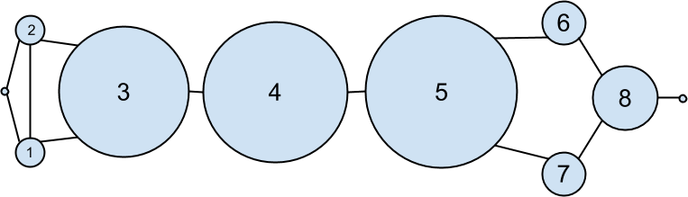
Figure 22-2. The DataSciencester network sized by betweenness centrality

Note

Generally the centrality numbers aren’t that meaningful themselves. What we care about is how the numbers for each node compare to the numbers for other nodes.

Another measure we can look at is closeness centrality. First, for each user we compute her farness, which is the sum of the lengths of her shortest paths to each other user. Since we’ve already computed the shortest paths between each pair of nodes, it’s easy to add their lengths. (If there are multiple shortest paths, they all have the same length, so we can just look at the first one.)

def farness(user_id: int) -> float:
    """the sum of the lengths of the shortest paths to each other user"""
    return sum(len(paths[0])
               for paths in shortest_paths[user_id].values())

after which it’s very little work to compute closeness centrality (Figure 22-3):

closeness_centrality = {user.id: 1 / farness(user.id) for user in users}

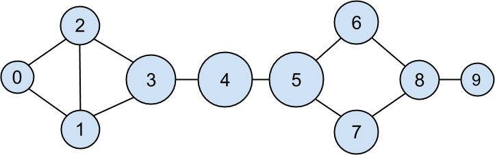
Figure 22-3. The DataSciencester network sized by closeness centrality

There is much less variation here—even the very central nodes are still pretty far from the nodes out on the periphery.

As we saw, computing shortest paths is kind of a pain. For this reason, betweenness and closeness centrality aren’t often used on large networks. The less intuitive (but generally easier to compute) eigenvector centrality is more frequently used.

Eigenvector Centrality

In order to talk about eigenvector centrality, we have to talk about eigenvectors, and in order to talk about eigenvectors, we have to talk about matrix multiplication.

Matrix Multiplication

If A is an $n\times m$ matrix and B is an $m\times k$ matrix (notice that the second dimension of A is same as the first dimension of B), then their product AB is the $n\times k$ matrix whose (i,j)th entry is:

$$A_{i1}{B}_{1j}+A_{i2}{B}_{2j}+\cdots +A_{im}{B}_{mj}$$

which is just the dot product of the ith row of A (thought of as a vector) with the jth column of B (also thought of as a vector).

We can implement this using the make_matrix function from Chapter 4:

from scratch.linear_algebra import Matrix, make_matrix, shape

def matrix_times_matrix(m1: Matrix, m2: Matrix) -> Matrix:
    nr1, nc1 = shape(m1)
    nr2, nc2 = shape(m2)
    assert nc1 == nr2, "must have (# of columns in m1) == (# of rows in m2)"

    def entry_fn(i: int, j: int) -> float:
        """dot product of i-th row of m1 with j-th column of m2"""
        return sum(m1[i][k] * m2[k][j] for k in range(nc1))

    return make_matrix(nr1, nc2, entry_fn)

If we think of an m-dimensional vector as an (m, 1) matrix, we can multiply it by an (n, m) matrix to get an (n, 1) matrix, which we can then think of as an n-dimensional vector.

This means another way to think about an (n, m) matrix is as a linear mapping that transforms m-dimensional vectors into n-dimensional vectors:

from scratch.linear_algebra import Vector, dot

def matrix_times_vector(m: Matrix, v: Vector) -> Vector:
    nr, nc = shape(m)
    n = len(v)
    assert nc == n, "must have (# of cols in m) == (# of elements in v)"

    return [dot(row, v) for row in m]  # output has length nr

When A is a square matrix, this operation maps n-dimensional vectors to other n-dimensional vectors. It’s possible that, for some matrix A and vector v, when A operates on v we get back a scalar multiple of v—that is, that the result is a vector that points in the same direction as v. When this happens (and when, in addition, v is not a vector of all zeros), we call v an eigenvector of A. And we call the multiplier an eigenvalue.

One possible way to find an eigenvector of A is by picking a starting vector v, applying matrix_times_vector, rescaling the result to have magnitude 1, and repeating until the process converges:

from typing import Tuple
import random
from scratch.linear_algebra import magnitude, distance

def find_eigenvector(m: Matrix,
                     tolerance: float = 0.00001) -> Tuple[Vector, float]:
    guess = [random.random() for _ in m]

    while True:
        result = matrix_times_vector(m, guess)    # transform guess
        norm = magnitude(result)                  # compute norm
        next_guess = [x / norm for x in result]   # rescale

        if distance(guess, next_guess) < tolerance:
            # convergence so return (eigenvector, eigenvalue)
            return next_guess, norm

        guess = next_guess

By construction, the returned guess is a vector such that, when you apply matrix_times_vector to it and rescale it to have length 1, you get back a vector very close to itself—which means it’s an eigenvector.

Not all matrices of real numbers have eigenvectors and eigenvalues. For example, the matrix:

rotate = [[ 0, 1],
          [-1, 0]]

rotates vectors 90 degrees clockwise, which means that the only vector it maps to a scalar multiple of itself is a vector of zeros. If you tried find_eigenvector(rotate) it would run forever. Even matrices that have eigenvectors can sometimes get stuck in cycles. Consider the matrix:

flip = [[0, 1],
        [1, 0]]

This matrix maps any vector [x, y] to [y, x]. This means that, for example, [1, 1] is an eigenvector with eigenvalue 1. However, if you start with a random vector with unequal coordinates, find_eigenvector will just repeatedly swap the coordinates forever. (Not-from-scratch libraries like NumPy use different methods that would work in this case.) Nonetheless, when find_eigenvector does return a result, that result is indeed an eigenvector.

Centrality

How does this help us understand the DataSciencester network? To start, we’ll need to represent the connections in our network as an adjacency_matrix, whose (i,j)th entry is either 1 (if user i and user j are friends) or 0 (if they’re not):

def entry_fn(i: int, j: int):
    return 1 if (i, j) in friend_pairs or (j, i) in friend_pairs else 0

n = len(users)
adjacency_matrix = make_matrix(n, n, entry_fn)

The eigenvector centrality for each user is then the entry corresponding to that user in the eigenvector returned by find_eigenvector (Figure 22-4).

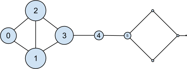
Figure 22-4. The DataSciencester network sized by eigenvector centrality

Note

For technical reasons that are way beyond the scope of this book, any nonzero adjacency matrix necessarily has an eigenvector, all of whose values are nonnegative. And fortunately for us, for this adjacency_matrix our find_eigenvector function finds it.

eigenvector_centralities, _ = find_eigenvector(adjacency_matrix)

Users with high eigenvector centrality should be those who have a lot of connections, and connections to people who themselves have high centrality.

Here users 1 and 2 are the most central, as they both have three connections to people who are themselves highly central. As we move away from them, people’s centralities steadily drop off.

On a network this small, eigenvector centrality behaves somewhat erratically. If you try adding or subtracting links, you’ll find that small changes in the network can dramatically change the centrality numbers. In a much larger network, this would not particularly be the case.

We still haven’t motivated why an eigenvector might lead to a reasonable notion of centrality. Being an eigenvector means that if you compute:

matrix_times_vector(adjacency_matrix, eigenvector_centralities)

the result is a scalar multiple of eigenvector_centralities.

If you look at how matrix multiplication works, matrix_times_vector produces a vector whose ith element is:

dot(adjacency_matrix[i], eigenvector_centralities)

which is precisely the sum of the eigenvector centralities of the users connected to user i.

In other words, eigenvector centralities are numbers, one per user, such that each user’s value is a constant multiple of the sum of his neighbors’ values. In this case centrality means being connected to people who themselves are central. The more centrality you are directly connected to, the more central you are. This is of course a circular definition—eigenvectors are the way of breaking out of the circularity.

Another way of understanding this is by thinking about what find_eigenvector is doing here. It starts by assigning each node a random centrality. It then repeats the following two steps until the process converges:

1. Give each node a new centrality score that equals the sum of its neighbors’ (old) centrality scores.

2. Rescale the vector of centralities to have magnitude 1.

Although the mathematics behind it may seem somewhat opaque at first, the calculation itself is relatively straightforward (unlike, say, betweenness centrality) and is pretty easy to perform on even very large graphs. (At least, if you use a real linear algebra library it’s easy to perform on large graphs. If you used our matrices-as-lists implementation you’d struggle.)

Directed Graphs and PageRank

DataSciencester isn’t getting much traction, so the VP of Revenue considers pivoting from a friendship model to an endorsement model. It turns out that no one particularly cares which data scientists are friends with one another, but tech recruiters care very much which data scientists are respected by other data scientists.

In this new model, we’ll track endorsements (source, target) that no longer represent a reciprocal relationship, but rather that source endorses target as an awesome data scientist (Figure 22-5).

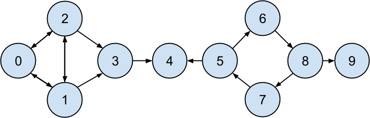
Figure 22-5. The DataSciencester network of endorsements

We’ll need to account for this asymmetry:

endorsements = [(0, 1), (1, 0), (0, 2), (2, 0), (1, 2),
                (2, 1), (1, 3), (2, 3), (3, 4), (5, 4),
                (5, 6), (7, 5), (6, 8), (8, 7), (8, 9)]

after which we can easily find the most_endorsed data scientists and sell that information to recruiters:

from collections import Counter

endorsement_counts = Counter(target for source, target in endorsements)

However, “number of endorsements” is an easy metric to game. All you need to do is create phony accounts and have them endorse you. Or arrange with your friends to endorse each other. (As users 0, 1, and 2 seem to have done.)

A better metric would take into account who endorses you. Endorsements from people who have a lot of endorsements should somehow count more than endorsements from people with few endorsements. This is the essence of the PageRank algorithm, used by Google to rank websites based on which other websites link to them, which other websites link to those, and so on.

(If this sort of reminds you of the idea behind eigenvector centrality, it should.)

A simplified version looks like this:

1. There is a total of 1.0 (or 100%) PageRank in the network.

2. Initially this PageRank is equally distributed among nodes.

3. At each step, a large fraction of each node’s PageRank is distributed evenly among its outgoing links.

4. At each step, the remainder of each node’s PageRank is distributed evenly among all nodes.

import tqdm

def page_rank(users: List[User],
              endorsements: List[Tuple[int, int]],
              damping: float = 0.85,
              num_iters: int = 100) -> Dict[int, float]:
    # Compute how many people each person endorses
    outgoing_counts = Counter(target for source, target in endorsements)

    # Initially distribute PageRank evenly
    num_users = len(users)
    pr = {user.id : 1 / num_users for user in users}

    # Small fraction of PageRank that each node gets each iteration
    base_pr = (1 - damping) / num_users

    for iter in tqdm.trange(num_iters):
        next_pr = {user.id : base_pr for user in users}  # start with base_pr

        for source, target in endorsements:
            # Add damped fraction of source pr to target
            next_pr[target] += damping * pr[source] / outgoing_counts[source]

        pr = next_pr

    return pr

If we compute page ranks:

pr = page_rank(users, endorsements)

# Thor (user_id 4) has higher page rank than anyone else
assert pr[4] > max(page_rank
                   for user_id, page_rank in pr.items()
                   if user_id != 4)

PageRank (Figure 22-6) identifies user 4 (Thor) as the highest-ranked data scientist.

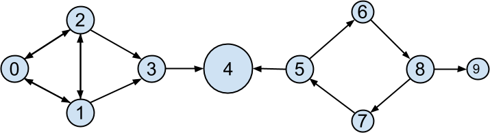
Figure 22-6. The DataSciencester network sized by PageRank

Even though Thor has fewer endorsements (two) than users 0, 1, and 2, his endorsements carry with them rank from their endorsements. Additionally, both of his endorsers endorsed only him, which means that he doesn’t have to divide their rank with anyone else.

For Further Exploration

• There are many other notions of centrality besides the ones we used (although the ones we used are pretty much the most popular ones).

• NetworkX is a Python library for network analysis. It has functions for computing centralities and for visualizing graphs.

• Gephi is a love-it/hate-it GUI-based network visualization tool.