Hierarchical Dynamic Neural Networks for Cascade System Modeling With Application to Wastewater Treatment
Wen Yu, DSc; Daniel Carrillo, DSc
Abstract
Many cascade processes, such as wastewater treatment, include complex nonlinear subsystems and many variables. The normal input–output relation only represents the first block and the last block of the cascade process.
In order to model the whole process, we use hierarchical dynamic neural networks to identify the cascade process. The internal variables of the cascade process are estimated. Two stable learning algorithms and theoretical analysis are given. Real operational data of a wastewater treatment plant are applied to illustrate this new neural modeling approach.
Keywords
Hierarchical neural networks; Cascade system; Wastewater treatment
1.1 Introduction
The input–output relation within a cascade process is very complex. It usually can be described by several nonlinear subsystems, as is for example the case with the cascade process of wastewater treatment. Obviously, the first block and the last block cannot represent the whole process. Hierarchical models can be used to model this problem. When the cascade process is unknown, only the input and output data are available. Black-box modeling techniques are needed. Also, the internal variables of the cascade process need to be estimated.
There are three different approaches that can be used to model a cascade process. If the input/output data in each subblock are available, each model is identified independently. If the internal variables are not measurable, a general method is to regard the whole process as one block and to use one model to identify it [6,3,19]. Another method is to use hierarchical models to identify cascade processes. Advantages of this approach are that the cascade information is used for identification and that the internal variable can be estimated. In [2], discrete-time feedforward neural networks are applied to approximate the uncertainty parts of the cascade system.
Neural networks can approximate any nonlinear function to any prescribed accuracy provided a sufficient number of hidden neurons can be incorporated. Hierarchical neural models consisting of a number of low-dimensional neural systems have been presented by [9] and [11] in order to avoid the dimension explosion problem. The main applications of hierarchical models are fuzzy systems, because rule explosion problem can be avoided in hierarchical systems [9], for example, in hierarchical fuzzy neural network [17], hierarchical fuzzy systems [12], and hierarchical fuzzy cerebellar model articulation controller (CMAC) networks [15]. Sensitivity analysis of the hierarchical fuzzy model was given in [12]. A statistical learning method was employed to construct hierarchical models in [3]. Based on Kolmogorov's theorem, [18] showed that any continuous function can be represented as a superposition of functions with the natural hierarchical structure. In [16], fuzzy CMAC networks are formed into a hierarchical structure.
The normal training method of hierarchical neural systems is still gradient descent. The key for the training of hierarchical neural models is to get an explicit expression of each internal error. Normal identification algorithms (gradient descent, least square, etc.) are stable under ideal conditions. They might become unstable in the presence of unmodeled dynamics. The Lyapunov approach can be used directly to obtain robust training algorithms of continuous-time and discrete-time neural networks. By using passivity theory, [5], [8], and [14] successfully proved that gradient descent algorithms of continuous-time dynamic neural networks were stable and robust to any bounded uncertainties.
The main problem for the training of a hierarchical neural model is the estimation of the internal variable. In this chapter, a hierarchical dynamic neural network is applied to model wastewater treatment. Two stable training algorithms are proposed. A novel approximate method for the internal variable of the cascade process is discussed. Real application results show that the new modeling approach is effective for this cascade process.
1.2 Cascade Process Modeling Via Hierarchical Dynamic Neural Networks
Each subprocess of a cascade process, such as wastewater treatment, can be described using the following general nonlinear dynamic equation:
where ![]() is the inner state,
is the inner state, ![]() is the input, and f is a vector function. Without loss of generality, we use two nonlinear affine systems to show how to use the hierarchical dynamic neural networks to model the system; see Fig. 1.1. The identified cascade nonlinear systems are given by
is the input, and f is a vector function. Without loss of generality, we use two nonlinear affine systems to show how to use the hierarchical dynamic neural networks to model the system; see Fig. 1.1. The identified cascade nonlinear systems are given by
where ![]() are the inner states of the subsystems, and
are the inner states of the subsystems, and ![]() ,
, ![]() ,
, ![]() , and
, and ![]() are unknown vector functions;
are unknown vector functions; ![]() can be also regarded as the output of subsystem 1 and as the input of subsystem 2;
can be also regarded as the output of subsystem 1 and as the input of subsystem 2; ![]() is the input of the whole system, and also the input of subsystem 1;
is the input of the whole system, and also the input of subsystem 1; ![]() is the output of the whole system, and also the output of subsystem 2.
is the output of the whole system, and also the output of subsystem 2.
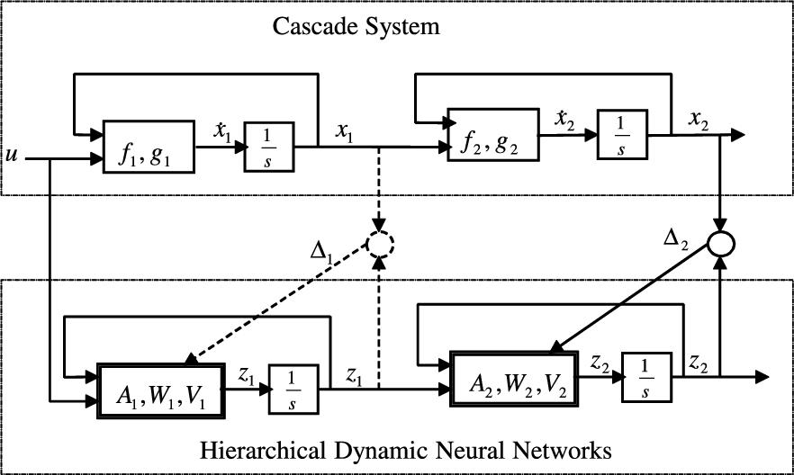
Only u and ![]() are available for the cascade process modeling. Since the internal variables are not measurable, a general method is to regard the whole process as one block and to use one model to identify it. Another method is to use hierarchical models to identify cascade processes. The advantages of this approach are that the cascade information is used for identification and that the internal variable can be estimated. In Section 1.3 we will show how to approximate it. In many wastewater treatment plants,
are available for the cascade process modeling. Since the internal variables are not measurable, a general method is to regard the whole process as one block and to use one model to identify it. Another method is to use hierarchical models to identify cascade processes. The advantages of this approach are that the cascade information is used for identification and that the internal variable can be estimated. In Section 1.3 we will show how to approximate it. In many wastewater treatment plants, ![]() is sampled occasionally. We can use this real value to improve the modeling accuracy.
is sampled occasionally. We can use this real value to improve the modeling accuracy.
We construct the following hierarchical dynamic neural networks to model (1.2):
where ![]() are the states of the neural models, and
are the states of the neural models, and ![]() ,
, ![]() ,
, ![]() , and
, and ![]() are the weights of the neural networks;
are the weights of the neural networks; ![]() and
and ![]() are known stable matrices. The active functions of
are known stable matrices. The active functions of ![]() and
and ![]() are used as sigmoid functions, i.e.,
are used as sigmoid functions, i.e.,
From Fig. 1.1, the modeling error is
The internal modeling error is
This will be estimated.
Generally, the hierarchical dynamic neural networks (1.3) cannot follow the nonlinear system (1.2) exactly. The nonlinear cascade system may be written as
where ![]() ,
, ![]() ,
, ![]() , and
, and ![]() are unknown bounded matrices. We assume the upper bounds,
are unknown bounded matrices. We assume the upper bounds, ![]() ,
, ![]() ,
, ![]() , and
, and ![]() , are known as
, are known as
where ![]() and
and ![]() are modeling errors and disturbances. Since the state and output variables are physically bounded, the modeling errors
are modeling errors and disturbances. Since the state and output variables are physically bounded, the modeling errors ![]() and
and ![]() can be assumed to be bounded too. The upper bounds of the modeling errors are
can be assumed to be bounded too. The upper bounds of the modeling errors are
where ![]() and
and ![]() are known positive matrices, and
are known positive matrices, and ![]() and
and ![]() are any positive definite matrices.
are any positive definite matrices.
Now we calculate the following errors:
where ![]() ,
, ![]() . Similarly,
. Similarly,
Because ![]() and
and ![]() are chosen as sigmoid functions, they satisfy the following Lipschitz property:
are chosen as sigmoid functions, they satisfy the following Lipschitz property:
where ![]() ,
, ![]() ,
, ![]() ,
, ![]() ,
, ![]() , and
, and ![]() are positive definite matrices.
are positive definite matrices.
1.3 Stable Training of the Hierarchical Dynamic Neural Networks
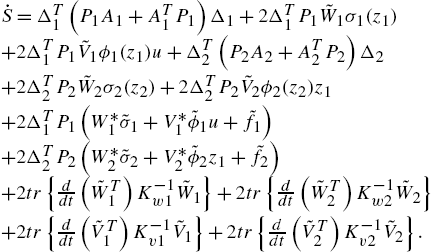
In order to obtain a stable training algorithm for the hierarchical dynamic neural networks (1.3), we calculate the error dynamics of the submodels. From (1.3) and (1.6), we have
If the outputs of all blocks are available, we can train each block independently via the modeling errors between neural models and the corresponding process blocks, ![]() and
and ![]() . Let us define
. Let us define
and the matrices ![]() and
and ![]() are selected to fulfill the following conditions:
are selected to fulfill the following conditions:
(1) the pair (![]() ) is controllable, the pair (
) is controllable, the pair (![]() ) is observable;
) is observable;
(2) if the local frequency condition [1] is satisfied, i.e.,
then the following assumption can be established.
A1: There exist a stable matrix ![]() and a strictly positive definite matrix
and a strictly positive definite matrix ![]() such that the matrix Riccati equation
such that the matrix Riccati equation
has a positive solution ![]() .
.
This condition is easily fulfilled if we select ![]() as a stable diagonal matrix. The next theorem states the learning procedure of a neuroidentifier. Similarly, there exist a stable matrix
as a stable diagonal matrix. The next theorem states the learning procedure of a neuroidentifier. Similarly, there exist a stable matrix ![]() and a strictly positive definite matrix
and a strictly positive definite matrix ![]() such that the matrix Riccati equation
such that the matrix Riccati equation
where ![]() ,
, ![]() .
.
First, we may choose ![]() and
and ![]() such that the Riccati equation (1.14) has a positive solution
such that the Riccati equation (1.14) has a positive solution ![]() . Then
. Then ![]() may be found according to the condition (1.8). Since (1.7) is correct for any positive definite matrix, (1.8) can be established if
may be found according to the condition (1.8). Since (1.7) is correct for any positive definite matrix, (1.8) can be established if ![]() is selected as a small enough constant matrix. The condition (1.8) has no effect on the network dynamics (1.3) and its training (1.16).
is selected as a small enough constant matrix. The condition (1.8) has no effect on the network dynamics (1.3) and its training (1.16).
Since the updating rates in (1.16) are ![]() , and
, and ![]() can be selected as any positive matrix, the learning process of the dynamic neural network is free of the solution of the Riccati equation (1.14).
can be selected as any positive matrix, the learning process of the dynamic neural network is free of the solution of the Riccati equation (1.14).
For many cascade systems the outputs in the internal blocks are not measurable, for example ![]() . The modeling error in the final block
. The modeling error in the final block ![]() should be propagated to the other blocks, i.e., we should calculate the internal modeling error
should be propagated to the other blocks, i.e., we should calculate the internal modeling error ![]() from
from ![]() .
.
From (1.3) and (1.6), the last block can be written as
where ![]() is the modeling error corresponding to the weights W and
is the modeling error corresponding to the weights W and ![]() . So
. So
So ![]() is approximated by
is approximated by
In Fig. 1.1 we note ![]() is the difference between the block “
is the difference between the block “![]() ” and the block “
” and the block “![]() .” So
.” So ![]() can be estimated as
can be estimated as
Here
where ![]() is the differential approximation error. So
is the differential approximation error. So
The internal modeling error is approximated by
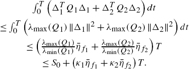
In order to ensure ![]() is bounded, we use (1.24) when
is bounded, we use (1.24) when ![]() . Otherwise, we use
. Otherwise, we use ![]() to represent
to represent ![]() , i.e.,
, i.e., ![]() .
.
Although the gradient algorithm (1.16) can ensure the modeling errors ![]() and
and ![]() are bounded (Theorem 1.1), the structure uncertainties
are bounded (Theorem 1.1), the structure uncertainties ![]() and
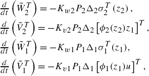
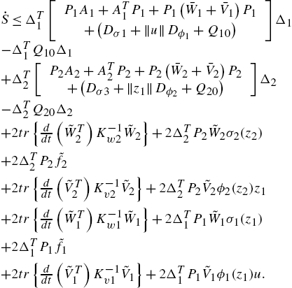
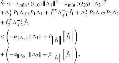
and ![]() will cause the parameters drift for the gradient algorithm (1.16). Some robust modification should be applied to make the parameters (weights) stable. In order to guarantee the overall models are stable, we use the following dead-zone training algorithm.
will cause the parameters drift for the gradient algorithm (1.16). Some robust modification should be applied to make the parameters (weights) stable. In order to guarantee the overall models are stable, we use the following dead-zone training algorithm.
1.4 Modeling of Wastewater Treatment
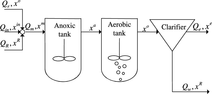
The wastewater treatment plant studied in this chapter is an anoxic/oxidant nitrogenous removal process [10]. It consists of two biodegradation tanks and a secondary clarifier in series form; see Fig. 1.2. Here, ![]() , and
, and ![]() denote flow of wastewater to be disposed, flow of mixed influent, flow of internal recycles, flow of external recycles, and flow of surplus sludge, respectively. Water quality indices such as chemical oxygen demand (COD), biological oxygen demand (BOD5), NH4-N (ammonia), nitrate, and suspended solid (SS) are decomposed into those components in activated sludge models (ASMs) [4]. The state variable x is defined as
denote flow of wastewater to be disposed, flow of mixed influent, flow of internal recycles, flow of external recycles, and flow of surplus sludge, respectively. Water quality indices such as chemical oxygen demand (COD), biological oxygen demand (BOD5), NH4-N (ammonia), nitrate, and suspended solid (SS) are decomposed into those components in activated sludge models (ASMs) [4]. The state variable x is defined as
where ![]() is soluble inert and
is soluble inert and ![]() is readily biodegradable substrate,
is readily biodegradable substrate, ![]() is suspended inert and
is suspended inert and ![]() is slowly biodegradable substrate,
is slowly biodegradable substrate, ![]() is suspended inert products,
is suspended inert products, ![]() is autotrophic biomass,
is autotrophic biomass, ![]() is heterotrophic biomass,
is heterotrophic biomass, ![]() is nitrate,
is nitrate, ![]() is ammonia,
is ammonia, ![]() is soluble oxygen,
is soluble oxygen, ![]() is soluble organic nitrogen,
is soluble organic nitrogen, ![]() is suspended organic nitrogen, and
is suspended organic nitrogen, and ![]() is alkalinity. In this tank, there are three major reaction processes, i.e.,
is alkalinity. In this tank, there are three major reaction processes, i.e.,
where COD represents carbonous contamination and AS denotes activated sludge. Nitrite is recycled from the aerobic tanks. It is deoxidized by autotrophic microorganisms in the denitrification phase by the following reaction:
The water quality index COD depends on the control input
and on the influent quality ![]() , i.e.,
, i.e.,
COD is also affected by other external factors such as temperature, flow distribution, and toxins. It is very difficult to find the nonlinear function ![]() [13].
[13].
We know each biological reactor in wastewater treatment plants can be described by the following dynamic equation:
where ![]() is the inner state, which is defined in (1.29),
is the inner state, which is defined in (1.29), ![]() is the input, which is defined in (1.32), φ denotes the reaction rates,
is the input, which is defined in (1.32), φ denotes the reaction rates, ![]() ,
, ![]() , and
, and ![]() .
.
The resulting steady-state values of anoxic and aerobic reactors are shown in Table 1.1. Used data are from 2003.
Table 1.1
Steady-state values of anoxic and aerobic reactors.
| S S | X BH | X S | X I | S NH | S I | S ND | X ND | S O | X BA | S NO | X P | S alk | |
|---|---|---|---|---|---|---|---|---|---|---|---|---|---|
| Anoxic | 1.2518 | 3249 | 74.332 | 642.4 | 7.9157 | 38.374 | 0.7868 | 5.7073 | 0.0001 | 220.86 | 3.9377 | 822.19 | 4.9261 |
| Aerobic | 0.6867 | 3244.8 | 47.392 | 643.36 | 0.1896 | 38.374 | 0.6109 | 3.7642 | 1.4988 | 222.39 | 12.819 | 825.79 | 3.7399 |

As discussed above, hierarchical dynamic neural networks are suitable for modeling this process. Each neural network corresponds to a reaction rate in a reactor, i.e.,
The design choices are as follows: both neural networks have one hidden layer, each hidden layer has 50 hidden nodes. The training algorithms of each neural model are (1.16); here the activation function ![]() ,
, ![]() , and the initial weights of
, and the initial weights of ![]() and
and ![]() are random numbers between
are random numbers between ![]() .
.
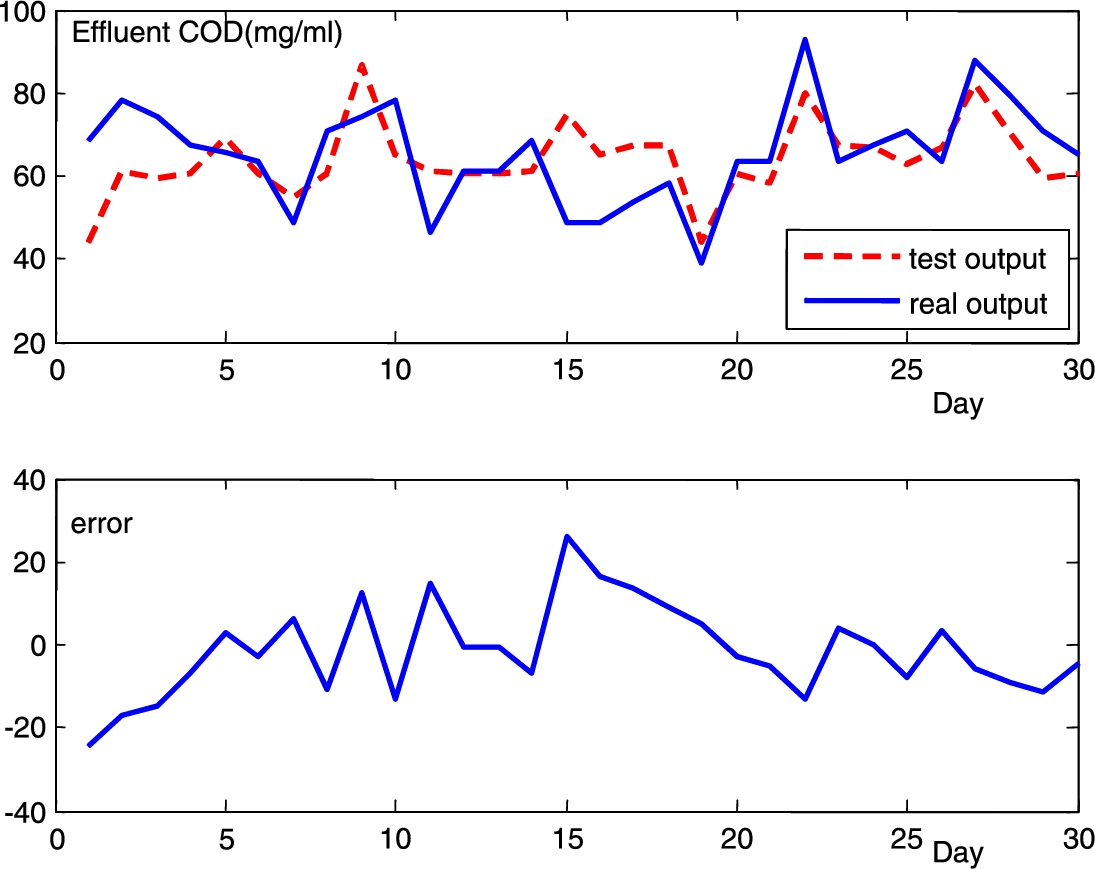
Dynamic modeling uses the steady-state values resulting from steady-state simulations as initial values with a hydraulic residence time of 10.8 h and a sludge age of 15 days. A total of 100 input/output data pairs from the records of 2003 are used as the training data, the other 30 input/output pairs as the testing data. The testing results of effluent COD are shown in Fig. 1.3.
We compare the hierarchical neural networks (HNNs) with the other three modeling methods, i.e., ASMs [4], linear models (LMs) [7], and neural networks (NNs) [6]. The model parameters of the ASM are the default values in [4]. The numbers of concerned variables in linear models are selected 2, 3, and 4. The hidden nodes of NNs are chosen as 30, 50, and 70; they are the same as those in the HNN. The initial values for all weights are chosen randomly from the interval ![]() . The comparison results are shown in Table 1.2, where the root mean square (RMS) of the HNN refers to the summation of errors in the final output.
. The comparison results are shown in Table 1.2, where the root mean square (RMS) of the HNN refers to the summation of errors in the final output.
Table 1.2
Comparison results of an activated sludge model (ASM), linear model (LM), neural network (NN), and hierarchical neural network (HNN). RMS, root mean square.
| Network | ASM | LM | NN | HNN | ||||
|---|---|---|---|---|---|---|---|---|
| Case | – | 2 | 4 | 30 | 50 | 70 | 10 | 70 |
| Parameters | 19 | 3 | 5 | 60 | 100 | 140 | 140 | 980 |
| Training | 148 | 0.1 | 0.21 | 3.8 | 5.28 | 5.23 | 2.73 | 36.81 |
| RMS | 37 | 11.99 | 11.54 | 24.39 | 8.45 | 10.64 | 11.81 | 8.62 |

The wastewater treatment process suffers from external disturbances such as temperature, influent qualities, influent flow, operational status, and internal factors like microorganism activities. Both the NN and the HNN can achieve high modeling accuracy. The LM and the NN can provide the water quality in the aerobic reactor, while the ASM and the HNN give water qualities in both anoxic and aerobic reactors.
1.5 Conclusions
The main contribution of this chapter is that a new hierarchical model is proposed. This hierarchical dynamic neural network is effective for cascade process modeling. Two stable training algorithms are discussed for this model. A new estimation method for the internal variables of the cascade process is illustrated. Real data of a wastewater treatment plant are applied to illustrate the modeling approach.


