Chapter 10

Sensitivity Analysis With Artificial Neural Networks for Operation of Photovoltaic Systems

O. May Tzuc, MEng; A. Bassam, PhD; L.J. Ricalde, PhD; E. Cruz May, MEng    

Abstract

One of the main disadvantages of artificial neural networks is their inability to provide a physical representation of what happens inside their hidden layers. This has categorized them, in most of the occasions, as black-box models, limiting their use exclusively to the establishment of relationships between input and output variables, ignoring the internal process. In the present chapter, a perspective of the use of sensitivity analysis of artificial neural networks is offered. Sensitivity analysis represents a powerful tool that allows us to solve this problem, granting new skills to artificial neural network models that can be exploited in various areas, ranging from decision making in operating processes to optimization. In this chapter, the sensitivity analysis will be described, its relevance, and the procedure to implement it in artificial neural networks, starting from the case study of temperature estimation in photovoltaic modules.

Keywords

Global sensitivity analysis; Elementary effect test; Computational modeling; Sensitivity convergence criteria

10.1 Introduction

In terms of energy and sustainability, photovoltaic (PV) systems are one of the most mature technologies for the use of solar resources. They offer a direct conversion of solar energy into electricity without moving parts and without producing atmospheric emissions [1]. On PV modules, the high levels of irradiance favor the generation of electrical energy; however, due to climatic conditions, the radiation at peak sun hours implies a negative impact on the electrical conversion efficiency [5]. For a typical commercial PV module operating at its maximum power point, only 10 to 15% of the incident light is converted into electricity, which means that a large part of the energy is converted into heat. Prolonged exposure to radiation increases the photon flow into the PV cells, resulting in the increase of the PV module temperature to values higher than the environmental temperature [15]. This causes the band gap of the PV semiconductor to shrink, increasing the short-circuit current of the module. However, the greatest effect that occurs in these conditions is the reduction in the open circuit voltage, causing the power, the form factor, and the performance also to reduce. Therefore, an increase in the operating temperature of the PV module reduces its efficiency, so it is necessary to extract as much energy as possible from the system to make it effective [30,29]. This leads to the need to develop strategies that counteract these adverse effects.

This type of problems is frequently found in various engineering branches, where it is required to establish the relationship between a given phenomenon and the parameters that influence it, in order to develop strategies that allow for decision making in operation processes, estimation of the phenomenon under certain conditions, and even the optimization of processes. The development of mathematical models provides a feasible solution for this type of situations. Mathematical models are a process of encoding and decoding of reality, in which a natural phenomenon is reduced to a formal numerical expression by a casual structure [24]. The modeling methods can be classified into statistical methods and heuristic methods (Fig. 10.1). The first are based on rigorous analysis of the interaction variables. They are the most widespread in the literature; however, they also turn out to be the most difficult to perform since a complete understanding of the interactions between the variables is required. On the other hand, heuristic methods are designed to establish an interaction between variables without a deep knowledge of the problem's physics, so they are commonly known as black-box models. The reason why the latter have experienced great growth in recent years is its quick implementation, making them one of the most popular of the artificial neural networks (ANNs).

Fig. 10.1 Process of modeling and classification.

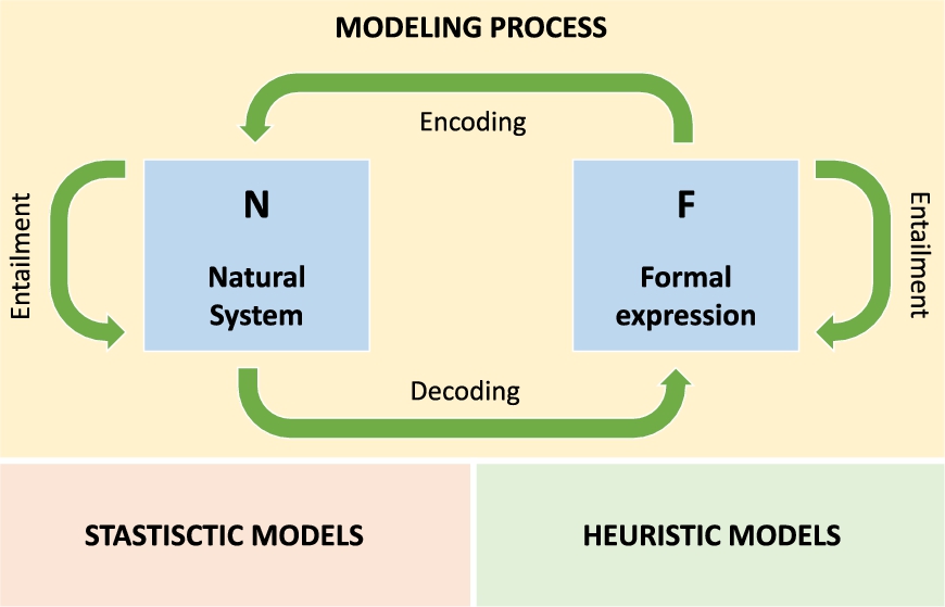
The main disadvantage of the use of ANNs is their inability to realize an analysis of the importance of input variables on the model output [17]. Contrary to the statistical models, where the influence of each independent variable is expressed by the estimated coefficients of the model, the output of ANN models cannot be explained directly [28]. This is because in most occasions the hidden layer of ANNs is considered a black box. Nevertheless, in this scenario, the statistical techniques of sensitivity analysis are presented as an adequate complement for the study of artificial intelligence models such as ANNs, since among other things, they allow understanding of the nature of the internal representations generated by the network to respond to a given problem, demystifying the black-box concept.

In this chapter, the use of a global sensitivity analysis technique applied to multilayer neural networks is shown, using as a case study the prediction of temperature in the operation of a photovoltaic system. The tool proposed in this chapter represents a power complement for the artificial intelligence modeling since it provides a broader perspective in the interpretation of the results obtained in the so-called black-box models.

10.2 Experimental Facility and Database

A PV array installation comprised of monocrystalline PV Siemens SR100 panels and an electric dual-axis solar tracking system are used for the study case presented in this chapter. The experimental facility is located in Mérida, Mexico. This city has a warm humid climate; its latitude and longitude are 20^∘ 58' N and 89^∘ 37' W, respectively.

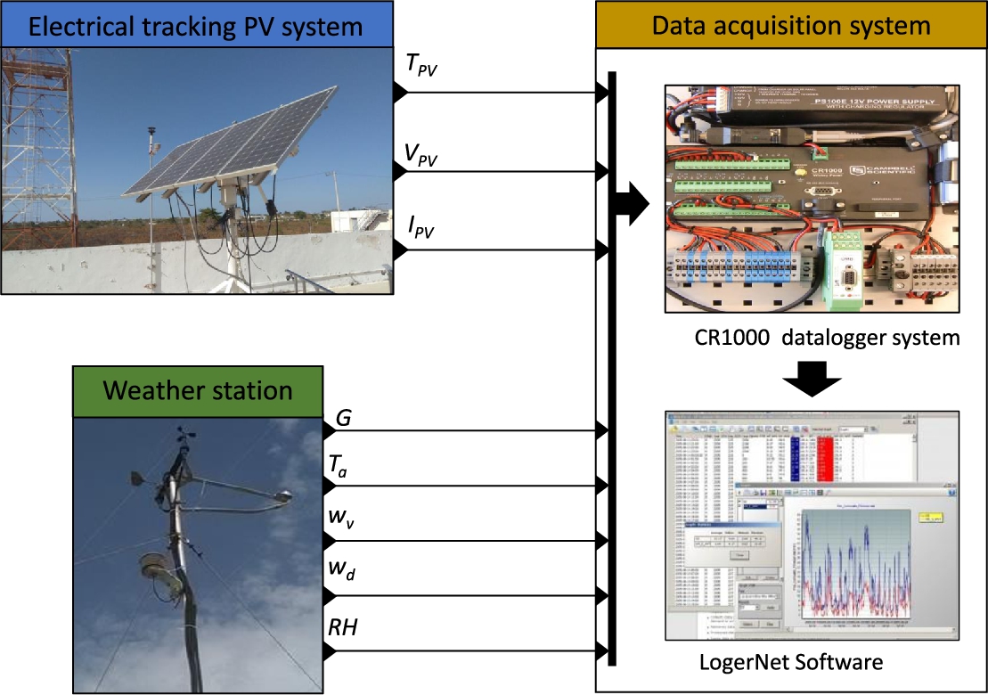
The experimental facility is equipped with sensors for the monitoring of meteorological variables, operating variables, and the temperature of the PV modules. Table 10.1 shows the sensed parameters and the characteristics of the measuring devices used for the collection of experimental data. A meteorological station was placed in the vicinity of the experimental system to consider the direct effects of the environmental variables, i.e., environment temperature, wind direction, wind speed, and relative humidity. In addition, a pyranometer was mounted on the tracking structure to sense the overall global radiation that acts directly on the PV surface [22,14]. To measure the PV temperature, infrared temperature sensors are placed in contact with the PV panels' backside [12], where the mean of the PV array is used as the dependent variable. Finally, PV power data are indirectly calculated by the measured PV voltage and PV current.

Table 10.1

Measured variables and instrumental equipment for the experimental database generation.

Measured variable		Sensor	Uncertainty
Global solar radiation	(G)	Campbell CS300-L Pyrometer	±5.00%
Environmental temperature	(Ta)	Campbell CS215-L	±4.00%
Wind velocity	(wv)	WINDSONIC4-L	±2.00%
Wind direction	(wd)	WINDSONIC4-L	±3.00%
Relative humidity	(RH)	Campbell CS215-L	±4.00%
PV voltage	(VPV)	TI LM747	±5.00%
PV current	(IPV)	FW BELL NT-50	±0.30%
PV temperature	(TPV)	Sensor K-Type	±0.80%

The experimental database contains measurements made over a course of 3 years, collected every 30 minutes by a Campbell Scientific CR1000 datalogger. Fig. 10.2 shows a diagram with the experimental facility and the sample acquisition process.

Fig. 10.2 Schematic diagram of the experimental facility designed to collect the case study database.

10.3 Sensitivity Analysis

Sensitivity analysis corresponds to a set of statistical techniques focused on determining how the variations of the M input variables (xi=x1,x2,…,xM) of a mathematical model influence the response value (yk). There are several reasons why sensitivity analysis is considered a necessary part in the development of computational models, specifically those based on artificial intelligence, including the following [9]:

• •  It allows to identify the order of importance that the input variables have for the output value generated by a mathematical model. This information is useful when one intends to use models based on ANNs as objective functions in optimization processes. This way it is possible to determine the feasibility of the optimization and to select in an appropriate way the operation variables that have the greatest impact on the process.
• •  It helps to identify variables that may need more research to improve the reliability of the model, because the ANNs are designed to establish correlations between dependent and independent variables without any notion of the nature of the data. By the analysis, it is possible to quickly evaluate various hypotheses of variables that are considered influential and determine their possible relevance, facilitating decision making in future studies (inverse process).
• •  It allows to identify the input variables that are insignificant for the model. In addition to knowing the range of importance of the input variables, the sensitivity analysis also identifies those that are not computationally relevant in the model. Therefore, these variables can be omitted, simplifying the computational model and reducing the computation time. This can be considered as an optimization process of the same mathematical model.
• •  It is helpful to determine if certain groups of input variables interact with each other. Some sensitivity analysis techniques allow us to identify how the input variables are affected by their mutual interaction. This interaction is useful at the moment of decision making to eliminate a variable from the computational model.
• •  It is useful when making decisions and identifying critical values. Since the ANN models are the product of the training and learning of experimental measurements, they are limited to operate between the maximum and minimum values of the input variables. Therefore, using sensitivity analysis it is possible to quantitatively know the acceptable limits for which the ANN model is functional.
• •  It helps to identify the coherence of the model with the real world and determine if the relationship is adequate. This is the most relevant point for ANN models, and artificial intelligence in general, because by its heuristic nature, sensitivity analysis serves as a tool to determine the adaptation of the model to the phenomenon under study, demystifying the black-box concept.

The above implies that at present the sensitivity analysis represents a vital element in the process of construction of ANN computational models. In order for a sensitivity analysis study to guarantee the correct reliability of its results, the method must meet the following specifications [24]:

• •  The method must be able to diagnose the effect of the input parameters, either individually or together.
• •  The method should test the influence of the input variables over the entire range.
• •  The method must be independent of the model.
• •  The method must be computationally efficient.
• •  The method must be applicable to discrete and continuous cases.

10.3.1 Sensitivity Analysis Classification

The literature reports various methods to carry out sensitivity analysis which can be grouped in different ways. However, one of the simplest ways to classify these methods is dividing them by the type of analysis performed and/or the type of interpretation of the results. As shown in Fig. 10.3, when the classification is made based on the type of analysis, it can be subdivided into local sensitivity analysis (LSA) and global sensitivity analysis (GSA) [10,4]. The ASL implementation requires the modeler to specify a nominal or reference value X¯ for the input variables. Thus, the variability of the model is given by the modification of each input value around the nominal value. On the other hand, GSA considers the variations of the entire possible ranges of values for the input variables [25,21]. Unlike LSA, GSA overcomes this possible limitation, but it still requires specifying the input variability space.

Fig. 10.3 Diagram of sensitivity analysis classification.

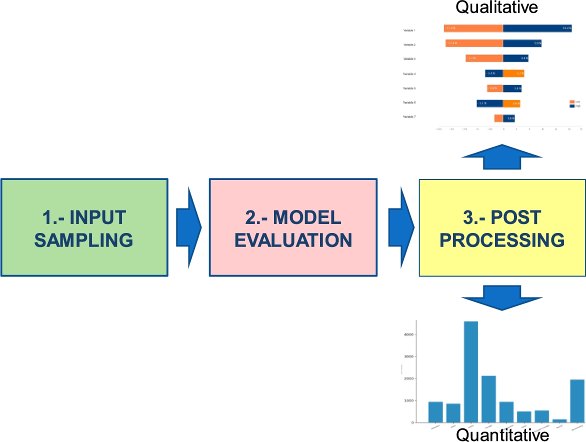
When the classification is conducted by the interpretation of results, it can be subdivided into quantitative and qualitative sensitivity analysis [26]. In qualitative sensitivity analysis, the sensitivity is assessed by visual inspection of model predictions or by visual tools (specialized plots) such as tornado plots and scatter plots. On the contrary, quantitative sensitivity analysis focuses on presenting numerical values that represent the sensitivity index of the variables. Quantitative sensitivity analysis can be complemented with visual tools that help in its interpretation.

Regardless of the method used, all of them are governed by three essential steps for the computation of sensitivity. As indicated in Fig. 10.4, the first step consists in the generation of random samples for the input variables. In the second step, the random samples are evaluated in the computational model in order to obtain the response of the model to the perturbations. Finally, a postprocessing analysis is performed, where the results are analyzed quantitatively or qualitatively, depending on the case, in order to define the sensitivity of each variable.

Fig. 10.4 Mandatory step to carry out a sensitivity analysis.

In this chapter we will focus on the study of one of the most versatile global sensitivity analysis techniques, known as the elementary effect test (EET). The following section aims to describe in a practical way this method of sensitivity analysis for its simple implementation in the environment of modeling engineering and artificial intelligence.

10.3.2 Elementary Effect Test

The EET is a GSA technique proposed by Morris [18] with low computation times, which makes it suitable for complex computational models such as ANNs. This technique allows ranking the importance of the input variables of a mathematical model in a simple way by using the so-called effective elements (EEs).

The EET works under the one-factor-at-a-time (OAT) concept, where the perturbations in the mathematical model are induced by varying one input factor at a time, keeping the other variables fixed. Fig. 10.5 illustrates the procedure for the generation of the EEs. In the first instance, a total of r random samples is generated for each input variable of the ANN model by applying numerical method techniques such as Monte Carlo or the Latin hypercube. The distribution of random samples is determined by the probability function used in sampling. The probability functions are chosen according to the nature of the input variable, where the most common are the uniform distribution function, the normal distribution function, and the Weibull distribution function. Subsequently, the random samples are grouped into data sets generating an M×r matrix of input variables. Each set of input variables (xi=x1,x2,…,xM) is altered one element at a time by a defined perturbation value Δ. As can be seen in Fig. 10.5, by this alteration, for each set of input variables, M additional sets are generated. Therefore, the total number of ANN model evaluations are given by

N = r ( M + 1 ) .

(10.1)

Fig. 10.5 Computational procedure for the generation of effective elements.

According to Fig. 10.5, once the N data set has been evaluated in the ANN model, the model responses to perturbations of the input variables are obtained. From these results it is possible to determine the EEs, considering the undisturbed date sets as baseline points (Xj). In general it can be indicated that the EE of the ith input factor xi at a given baseline point Xj and for a predefined perturbation is given by [13]

E E i j = y ( x 1 j , x 2 j , . . . , x i j + Δ , . . . x j M ) − y ( x 1 j , x 2 j , . . . , x i j , . . . x M j ) Δ .

(10.2)

Thus, the EEs quantify how much the ANN result is affected by the disturbance in the ith variable, where the total number of EEs is r per variable. The EEs' average value (μi) is considered the sensitivity measure for the ith input parameter. In order to avoid compensation by negative values, the mean of the absolute values of EEs (μi⁎) is used [7], i.e.,

μ i ⁎ = 1 r ∑ j = 1 r | E E i j | .

(10.3)

On the other hand, as a secondary product of this analysis the intensity of the interaction of the ith input parameter with respect to another input parameter can be interpreted from the standard deviation of EEs (σi), i.e.,

σ i = 1 r ∑ j = 1 r ( E E i j − μ i ) 2 .

(10.4)

10.3.3 Elementary Effect Test Visualization

In order to establish a first immediate interpretation of the results by the sensitivity analysis method, the EET relies on two types of graphs, i.e., the EET plot and the convergence analysis plot, which provide different levels of information. An example of an EET plot is shown in Fig. 10.6. As can be seen, it is a bidimensional plot where the x-axis represents the mean absolute values of EEs (μ) and the y-axis represents the standard deviation of the EEs (σ) for each input variable. According to Fig. 10.6, on the x-axis, the greater the displacement of a variable towards the right, the greater the sensitivity or impact this variable will have on the output of the ANN model. Similarly, on the y-axis, the greater the upward displacement of a variable, the greater the influence it exerts on the other input variables. In the example of Fig. 10.6, it can be seen that a variable with a greater influence on the output of the model does not necessarily have the most influence among the input values, as seen with x3 and x5, as well as x1 and x4.

Fig. 10.6 Representation of an elementary effect test plot.

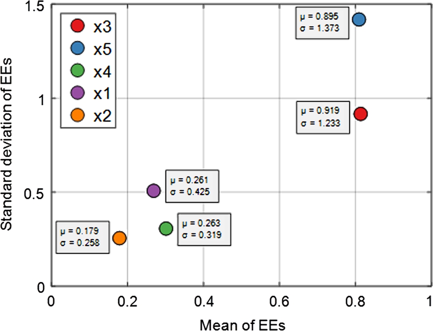
Fig. 10.7 illustrates an example of the convergence analysis plot. It estimates the sensitivity of each independent variable by systematically increasing the number of random samples (r) to be evaluated in the ANN model [20]. This type of visualization allows for verification that the sensitivity indices do not change, or vary slightly, when using different samples in the model evaluations, which are knowledge as convergence, guaranteeing the reliability of the results. In addition, it helps to determine the minimum number of r samples required for the sensitivity analysis of a given computational model.

Fig. 10.7 Convergence analysis plot representing the three levels of convergence.

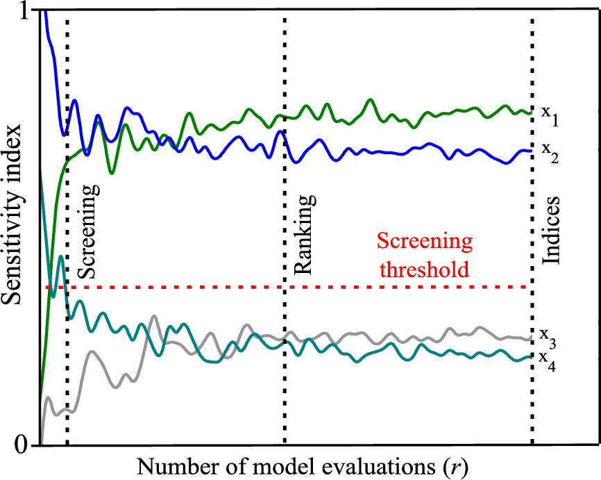
The literature reports that for an adequate interpretation of the convergence analysis it is necessary to classify the convergence of the sensitivity analysis at three levels: convergence of screening, convergence of ranking, and convergence of sensitivity indices [26,21]. Fig. 10.7 exemplifies the points in which each of the convergence levels is met through the vertical lines screening, ranking, and indices:

• •  The first convergence level to be detected is the screening. At this level, the variables of the model are classified into influential parameters and noninfluential parameters. This classification is made using a screening threshold, where the variables below it are not considered relevant for the mathematical model. The screening threshold value is determined by the modeler; the most common values are 0.05 and 0.01. The convergence of screening is reached when the partition among sensitive and insensitive variables (indices below the screening threshold) is stabilized.
• •  The second convergence level is the ranking. The ranking is used to know the order of importance of the input variables in the ANN model. From this point, the analysis will focus on determining the value of the sensitivity index of each variable. This level of convergence is sufficient when the purpose is to determine only the importance of the variables, as in the case of optimization problems. The convergence of ranking is achieved when the ordering among the variables remains stable.
• •  The last convergence level is the determination of the sensitivity indices. At this level, the numeric value of the sensitivity index for each input variable is defined. However, it requires evaluating a large number of random samples to obtain them, making this the level of convergence most complicated to achieve. The more accurate the sensitivity index is desired, the greater the number of random samples (r) that will have to be evaluated in the model. The convergence of sensitivity indices is achieved when the values of the indices remain stable or quasistable.

10.4 Application

10.4.1 Modeling and Sensitivity Analysis Workflow

A computational workflow is shown in Fig. 10.8 indicating the steps to carry out ANN modeling together with EET. This workflow is based on the case study for predicting the operating temperature of PV modules by using multilayer perceptron neural networks. According to the figure, the workflow is divided into two parts: the first one corresponds to the development of the ANN model, and the second one focuses on the evaluation of the model by GSA methods to obtain the sensitivity indices.

Fig. 10.8 Schematic workflow for the implementation of the EET with an ANN.

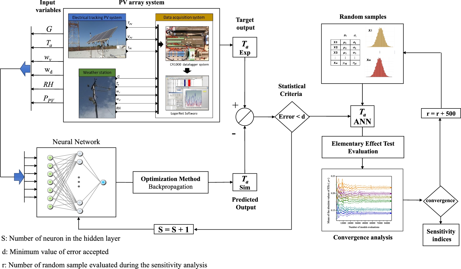
In Fig. 10.8, the experimental database to develop the ANN model is randomly divided in two parts: 80% is destined to ANN learning and testing and the remaining 20% is used for the validation of the model. This procedure guarantees an adequate distribution of the data and a good representation of the phenomenon under study. Once the database is divided, the learning process of the ANN is initiated. At this stage the database for training is normalized and entered into a basic ANN architecture, which is composed of M neurons in the input layer (the number of input variables), S neurons in the hidden layer (s), and k neurons in the output layer (the number of output variables). During the learning process, the ANN seeks to minimize the error between the estimated value and the experimental measurement by using optimization algorithms to adjust the weights and bias values, a technique commonly known as backpropagation [11]. When the learning process is completed, a statistical comparison between experimental data and ANN training/validation results is made. If it does not meet the criteria, the ANN architecture is modified more and the learning process is repeated. For the case study presented, Table 10.2 contains the ANN model parameter settings, such as the independent and dependent variables selected for the PV temperature modeling.

Table 10.2

Parameter settings and variables characteristic for the development of artificial neural network PV prediction models.

ANN parameter	Setting
Hidden neurons active function	Tangent sigmoidal [2]
Output neurons active function	Pureline [2]
Optimization algorithm	Levenberg–Marquardt [8]
Maximum number of iterations	1000
Number of input neurons (M)	6
Number of output neurons (k)	1

Variable		Min	Max	Unit
Inputs:
Global solar radiation	(G)	100	1367	[W/m2]
Environment temperature	(Ta)	10	40	[∘C]
Wind velocity	(wv)	0.22	9.85	[m/s]
Wind direction	(wd)	0	359	[∘]
Relative humidity	(RH)	27	98	[%]
PV power	(PPV)	16.8	332	[W]
Output:
PV temperature	(TPV)	12.7	66.4	[∘C]

The sensitivity analysis is performed using the best ANN model obtained in the learning process. In the sensitivity analysis r random samples are generated by each input variable, based on a designed probability distribution function. Afterwards, the random samples are evaluated in the ANN model developed to generate the r effective elements. The next step is to compute the sensitivity indices for EE from 1 to r and to analyze the fulfillment of the three levels of convergence by a convergence analysis plot. If the comparison does not satisfy the convergence of sensitivity indices, the number of samples r to be evaluated is increased and the process is repeated iteratively.

10.4.2 Artificial Neural Network

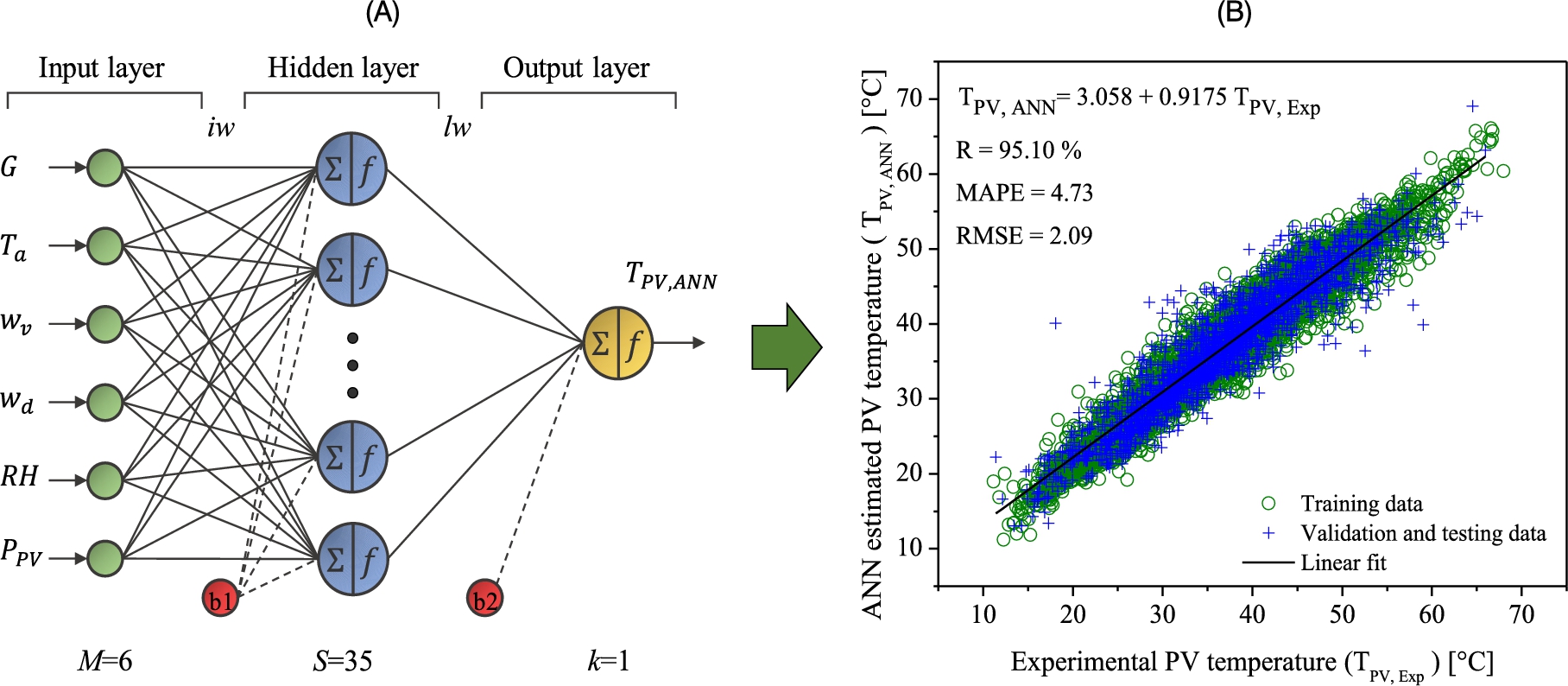
The best ANN architecture for estimation of the temperature of the photovoltaic modules was obtained using a trial-and-error approach by varying the number of neurons (S) in the hidden layer, as described in Section 10.4.1. As can be seen in Fig. 10.9A, the developed ANN prediction model consists of 35 neurons in the hidden layer and the transfer function pair tansig–purelin, generating a 6-35-1 ANN architecture. It is described by the mathematical function [6]

T P V , A N N = ∑ s = 1 S [ l w ( 1 , s ) ( 1 1 + exp ⁡ ( − 2 ( ∑ m = 1 M ( i w ( s , m ) x ( m ) ) + b 1 ( s ) ) ) ) + 1 ] + b 2 ,

(10.5)

where iw represents the weights from the input to the hidden layer, lw represents the weights from the hidden to the output layer, M is the total number of input neurons (M=6), S is the total number of hidden neurons (S=35), and b1 and b2 correspond to the bias values for the hidden and output neurons, respectively. This model was evaluated under the statistical parameters mean absolute percentage error (MAPE), root mean square error (RMSE), and coefficient of correlation (R2) [16]. The obtained results (MAPE = 3.48% and RMSE = 0.4541; the best linear behavior fitting with R2=98.48%) indicate that the model has a good prediction capacity with an accuracy above 93% (Fig. 10.9B).

Fig. 10.9 Convergence analysis plot representing the three levels of convergence.

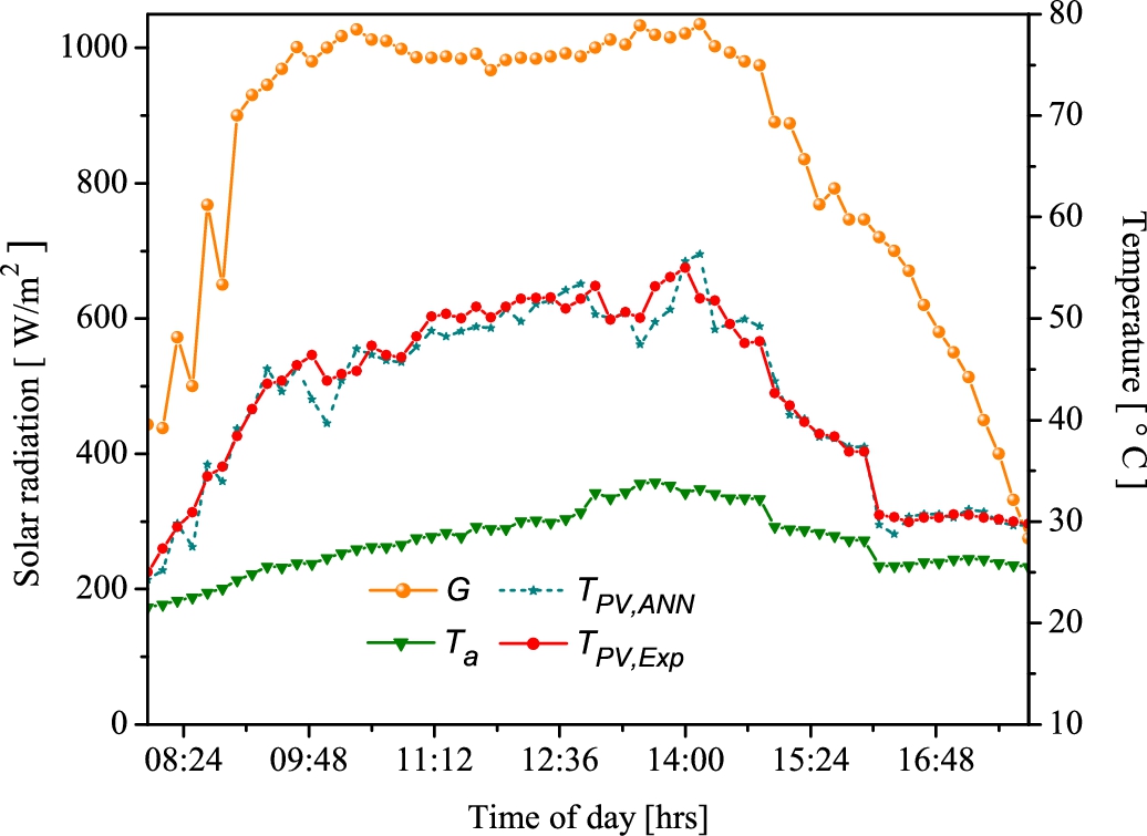
An adequate practice in modeling with ANNs is to validate the developed model comparing its results with experimental samples not included in the training and testing phases. In the present study case, this validation was carried out using data measurements corresponding to standard days at the experimental location. From Fig. 10.10, it can be seen that the developed model has a good adaptation to the changes in temperature recorded during the day.

Fig. 10.10 ANN model validation with data not included in the training and testing phase.

10.4.3 Sensitivity Analysis Results

To perform the sensibility analysis, it is necessary to consider the computational design set-up for the sampling of the variables and the convergence criteria. In this example, for the generation of the input variables, the uniform distribution function was selected using the normalized values present in Table 10.2 as function parameters. In addition, the sampling strategy used to proportionally distribute the random sample was the Monte Carlo method. On the other hand, a screening threshold of 0.1 and a maximum number of evaluated samples r equal to 100000 were taken as sensitivity analysis convergence criteria. Table 10.3 summarizes the selected settings for the sensitivity analysis.

Table 10.3

Sampling and convergence criteria set-up for the sensitivity analysis.

Sensitivity analysis set-up for sampling the parameter space
Parameter distribution	Uniform distribution
Design type	Radial
Sample strategy	Monte Carlo
Sensitivity analysis set-up for convergence analysis
Threshold value	1.0
Maximum number of samples evaluated (rmax)	100000

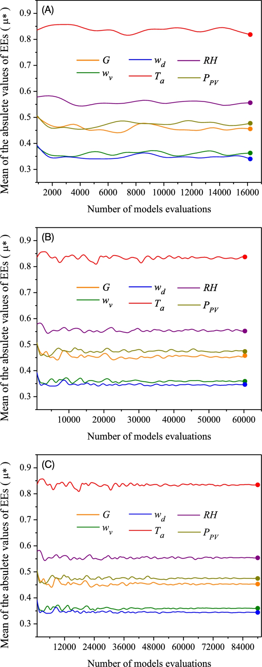
Applying the methodology described in the workflow of Fig. 10.9, the sensitivity indices for the several cases of r are calculated. Fig. 10.11 exemplifies the convergence analysis results for three different r values (16000, 60000, and 90000). Fig. 10.11A illustrates the case when 16000 samples are used. As can be seen in this figure, all the variables exceed the screening threshold assigned in Table 10.3; therefore it is considered that all are influential for the ANN model results. From this figure it is also distinguished that some parameters have to present a greater relevance in the model than others (Ta and RH). Nevertheless, according to the behavior of the convergence curves, the number of samples used does not indicate the general relevance of the variables. Fig. 10.11B shows the convergence analysis when r=60000. As can be seen, the increase in the number of samples evaluated in the ANN model significantly improves the behavior of the convergence curves. At this point it is easy to see that the convergence of ranking has been fulfilled. However, the sensitivity indices have not been established accurately for some variables, such as RH and Ta. Finally, Fig. 10.11C presents the analysis for r=90000. Similar to Fig. 10.11B, the increase in r reduces the disturbance in the sensitivity indices. From this point, it is observed that the disturbances in each sensitivity index are so insignificant that the values remain quasistable. Therefore, it can be concluded that this is the appropriate range for the case study that provides quantitative values of the sensitivity indices.

Fig. 10.11 Convergence analysis plots of the study case. (A) Convergence of screening achieved. (B) Convergence of ranking achieved. (C) Convergence of sensitivity indices achieved.

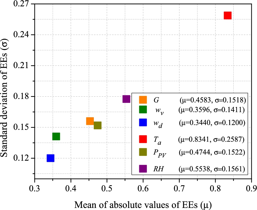
Once the convergence analysis with the three levels of convergence is satisfactorily concluded, it is possible to represent the results by an EET plot, as shown in Fig. 10.12. In this plot, it is seen that the ambient temperature is the parameter that has the greatest effect on the operating temperature of the PV module, and also the one that has the greatest influence on the other input variables. Also, from the analysis of the graph it is observed that although the solar radiation is less influential for the output of the model than the PV power, it has a greater impact on the input variables. Finally, the wind speed and direction are the parameters that contribute the least to the operating temperature of the module, according to the experimental measurements of the case study. Based on the case study, these results allow for identifying which variables affect the PV operation temperature to the greatest extent, and thus implementing the appropriate strategies to reduce their impact and improve their operation.

Fig. 10.12 Elementary effect test plots with the results of the case study.

10.5 Conclusions

In this chapter, the implementation of a method of GSA in multilayer perceptron ANNs is presented. Using as a case study the modeling of the operating temperature of a PV module under the meteorological conditions of a city in the Yucatan peninsula, a methodology was proposed to link together the GSA and ANNs. The global sensitivity analysis technique presented in this chapter corresponds to the EET method, which due to its rapid response time, ranking capacity, and quantifiable value generation represents a feasible option to be implemented in the analysis of ANNs. In order to present a systematic implementation process, a computational workflow is proposed to facilitate the reader's understanding and use of the proposed methodology. The end of the chapter indicates that the use of the EET in ANNs allows the modeler to develop more complex models and facilitates the decision making in terms of operation, optimization, and analysis of the model's physics. Finally, the methodology presented in the workflow can be easily extrapolated for the use of more complex GSA techniques reported in the literature by using simple modifications.

References

1. M. Bazilian, I. Onyeji, M. Liebreich, I. MacGill, J. Chase, J. Shah, D. Gielen, D. Arent, D. Landfear, S. Zhengrong, Re-considering the economics of photovoltaic power, Renewable Energy 2013;53:329–338.

2. M.H. Beale, M.T. Hagan, H.B. Demuth, Neural Network Toolbox™ User's Guide R2017a. The MathWorks, Inc.; 2017.

3. E. Borgonovo, E. Plischke, Sensitivity analysis: a review of recent advances, European Journal of Operational Research 2016;248(3):869–887.

4. E. Castillo, A.S. Hadi, A. Conejo, A. Fernández-Canteli, A general method for local sensitivity analysis with application to regression models and other optimization problems, Technometrics 2004;46(4):430–444. http://www.tandfonline.com/doi/abs/10.1198/004017004000000509.

5. E. Cruz May, L.J. Ricalde, E.J.R. Atoche, A. Bassam, E.N. Sanchez, Forecast and energy management of a microgrid with renewable energy sources using artificial intelligence, C. Brito-Loeza, A. Espinosa-Romero, eds. Intell. Comput. Syst.. Cham: Springer International Publishing; 2018:81–96.

6. Y. El Hamzaoui, M. Abatal, A. Bassam, F. Anguebes-Franseschi, O. Oubram, I. Castaneda Robles, O. May Tzuc, Artificial neural networks for modeling and optimization of phenol and nitrophenols adsorption onto natural activated carbon, Desalination and Water Treatment 2017;58:202–213.

7. L. Gao, B.A. Bryan, Incorporating deep uncertainty into the elementary effects method for robust global sensitivity analysis, Ecological Modelling 2016;321:1–9.

8. M.T. Hagan, M.B. Menhaj, Training feedforward networks with the Marquardt algorithm, IEEE Transactions on Neural Networks 1994;5(6):989–993.

9. J.W. Hall, S.A. Boyce, Y. Wang, R.J. Dawson, S. Tarantola, A. Saltelli, Sensitivity analysis for hydraulic models, Journal of Hydraulic Engineering 2009;135(11):959–969.

10. D.M. Hamby, A review of techniques for parameter sensitivity analysis of environmental models, Environmental Monitoring and Assessment 1994;32(2):135–154.

11. S. Haykin, Neural Networks. Upper Saddle River, NJ: Prentice Hall; 1999.

12. M. Jankovec, M. Topič, Intercomparison of temperature sensors for outdoor monitoring of photovoltaic modules, Journal of Solar Energy Engineering 2013;135(3), 031012. http://solarenergyengineering.asmedigitalcollection.asme.org/article.aspx?doi=10.1115/1.4023518.

13. L. Lee, P. Srivastava, G. Petropoulos, Overview of sensitivity analysis methods in Earth observation modeling, Sensitivity Analysis in Earth Observation Modelling. 2017:3–24. http://linkinghub.elsevier.com/retrieve/pii/B978012803011000001X.

14. L.H.I. Lim, Z. Ye, D. Yang, Non-contact measurement of POA irradiance and cell temperature for PV systems, IECON 2015 - 41st Annu. Conf. IEEE Ind. Electron. Soc.. 2015:386–391.

15. G. Makrides, B. Zinsser, M. Norton, G.E. Georghiou, M. Schubert, J.H. Werner, Potential of photovoltaic systems in countries with high solar irradiation, Renewable and Sustainable Energy Reviews 2010;14(2):754–762.

16. O. May Tzuc, A. Bassam, M. Abatal, Y. El Hamzaoui, A. Tapia, Multivariate optimization of Pb(II) removal for clinoptilolite-rich tuffs using genetic programming: a computational approach, Chemometrics and Intelligent Laboratory Systems Jun 2018;177:151–162 10.1016/j.chemolab.2018.02.010. http://linkinghub.elsevier.com/retrieve/pii/S0169743917306044.

17. J.J. Montano, A. Palmer, Numeric sensitivity analysis applied to feedforward neural networks, Neural Computing & Applications 2003;12(2):119–125. http://link.springer.com/10.1007/s00521-003-0377-9.

18. M.D. Morris, Factorial sampling plans for preliminary computational experiments, Technometrics 1991;33(2):161–174.

19. J. Nossent, P. Elsen, W. Bauwens, Sobol' sensitivity analysis of a complex environmental model, Environmental Modelling & Software 2011;26(12):1515–1525. http://www.sciencedirect.com/science/article/pii/S1364815211001939. http://www.sciencedirect.com/science/article/pii/S1364815211001939/pdfft?md5=a3e52e678ed8b2c2ca9cb2c613f039ea&pid=1-s2.0-S1364815211001939-main.pdf.

20. F. Pianosi, K. Beven, J. Freer, J.W. Hall, J. Rougier, D.B. Stephenson, T. Wagener, Sensitivity analysis of environmental models: a systematic review with practical workflow, Environmental Modelling & Software 2016;79:214–232 10.1016/j.envsoft.2016.02.008.

21. F. Pianosi, T. Wagener, A simple and efficient method for global sensitivity analysis based on cumulative distribution functions, Environmental Modelling & Software 2015;67:1–11 10.1016/j.envsoft.2015.01.004. http://www.sciencedirect.com/science/article/pii/S1364815215000237.

22. J. Polo, S. Garcia-Bouhaben, M.C. Alonso-García, A comparative study of the impact of horizontal-to-tilted solar irradiance conversion in modelling small PV array performance, Journal of Renewable and Sustainable Energy 2016;8(5).

23. M. Ratto, F. Campolongo, D. Gatelli, M. Saisana, Sensitivity analysis: from theory to practice, http://doi.wiley.com/10.1002/9780470725184.ch6; 2008 August 2015.

24. A. Saltelli, M. Ratto, T. Andres, F. Campolongo, J. Cariboni, D. Gatelli, M. Saisana, S. Tarantola, Global Sensitivity Analysis. The Primer, http://www.scopus.com/inward/record.url?eid=2-s2.0-84889461919&partnerID=40&md5=367cd0af66837fc6e4ae661b69007cd9; 2008.

25. A. Saltelli, P. Annoni, I. Azzini, F. Campolongo, M. Ratto, S. Tarantola, Variance based sensitivity analysis of model output. Design and estimator for the total sensitivity index, Computer Physics Communications 2010;181(2):259–270 10.1016/j.cpc.2009.09.018.

26. F. Sarrazin, F. Pianosi, T. Wagener, Global sensitivity analysis of environmental models: convergence and validation, Environmental Modelling & Software May 2016;79:135–152 10.1016/j.envsoft.2016.02.005.

27. W. Tian, A review of sensitivity analysis methods in building energy analysis, Renewable and Sustainable Energy Reviews Apr 2013;20:411–419. https://www.sciencedirect.com/science/article/pii/S1364032112007101.

28. C. Vasilakos, K. Kalabokidis, J. Hatzopoulos, I. Matsinos, Identifying wildland fire ignition factors through sensitivity analysis of a neural network, Natural Hazards 2009;50(1):125–143.

29. M.E. Ya'Acob, H. Hizam, T. Khatib, M.A.M. Radzi, C. Gomes, M. Bakri A., M.H. Marhaban, W. Elmenreich, Modelling of photovoltaic array temperature in a tropical site using generalized extreme value distribution, Journal of Renewable and Sustainable Energy 2014;6(3).

30. S. Zahurul, N. Mariun, M.L. Othman, H. Hizam, I. Zainal, A. Arash, Ambient temperature effect on Amorphous Silicon (A-Si) photovoltaic module using sensing technology, 2015 Ninth Int. Conf. Sens. Technol. Ambient. 2015:235–241.