Chapter 3
Design and Fabrication of Vibration-Induced Electromagnetic Microgenerators

3.1 Introduction

To develop energy devices that are more compactly renewable, MEMS technologies may be used. Using MEMS (microelectromechanical systems) to fabricate a microgenerator, the energy source can be retrieved by an electromechanical mechanism [1] used in sensor systems and networks for automotive, robotics, medical electronics, wearable computers, and household applications. In such applications, a self-powered device can be used for renewable energies obtained from the ambient environment, reduce pollutants on Earth, and provide an independent power source for a microsystem without requiring conventional solutions such as power supplies or batteries [2].

Many achievements in self-powered devices have been reported. In 2006, Beeby et al. [3] reviewed state-of-the-art self-powered microsystems and discussed MEMS technology developments in the context of microfabrication and design capabilities. These efforts have resulted in a wide variety of compact sensors and actuators. In 2007, Arnold [4] summarized the power density (PD) (W cm^–3) of some state-of-the-art generators, indicating that a PD exceeding 2 mW cm^–3 is possible for a compact magnetic power generation system.

Some researchers have used a commercially available finite-element code to examine the response of a resonating spring-mass system [5–10]. For example, in 2001, El-hami et al. [5] employed MATLAB® to predict the power output of an electromagnetic generator and used the computer-aided design (CAD) software package VF-OPERA to analyze the magnetic field distribution. Ching et al. [6], Shearwood and Yates [7], Williams et al. [8, 9], Beeby et al. [10], and Buren and Troster [11] used ANSYS to model the mechanical motion of a spring-mass system on an electromagnetic device with a magnet and a spring, and have investigated the results of voltage outputs within various governing vibration parameters.

El-hami et al. [5] used stainless steel sheets to manufacture a cantilever beam vibration spring, which is shown in Figure 3.1. The micromagnetic generator is composed of a vibration spring, a copper inducer coil, and a permanent magnet (PM) of neodymium-iron-boron (NdFeB). The volume and weight of this microgenerator are 240 mm³ and 500 mg, respectively. This microgenerator can operate at a resonant vibration frequency of 322 Hz and an amplitude of 25 µm; its mean-square-root voltage and power output are 12.8 mV and 53 µW, respectively, with a loading resistor of 0.28 Ω.

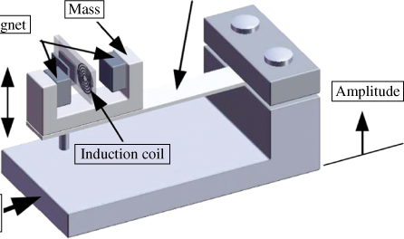
Figure 3.1 Schematic of a stainless steel canti-lever beam microgenerator

Amirtharajah and Chandrakasan [12] developed a tubular electro-magnetic microgenerator composed of a cylindrical spiral spring, a mass with an induction coil, and a PM, as shown in Figure 3.2. The vibration mass of this device weighs approximately 500 mg. An induced voltage of 0.18 V and a power output of 400 µW were obtained using an induction coil of 10 Ω under a vibration of amplitude 20 mm and frequency of c. 100 Hz.

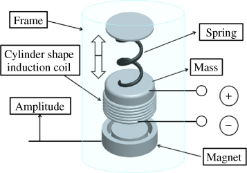
Figure 3.2 Schematic of an electromagnetic column-shape microgenerator

Li and colleagues [13] used laser-forming technology to manufacture a copper spiral microspring constituting a vibration-type electro-magnetic microgenerator with a volume of 1 cm³, which is shown in Figure 3.3. This device could generate a voltage of 2–4 V and a power output of 10 µW at a frequency of 200 Hz and an amplitude of less than 200 µm.

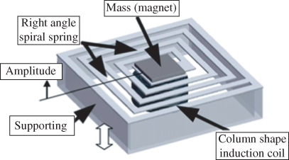
Figure 3.3 Schematic of copper spiral spring microgenerator

Pan et al. [14] used deep reactive ion etching (DRIE) technology and a silicon wafer to develop a spiral microspring on which a Ferro-platinum thin film is sputtered at its center. By combining a plane-type spiral induction coil, a thin-film vibration electromagnetic microgenerator was developed as shown in Figure 3.4. The volume and thickness are less than 0.34 cm³ and 0.34 mm, respectively. An induction voltage of 40 mV and a power output of 100 µW were obtained at a resonant frequency of 60 Hz and an amplitude of 0.03 mm.

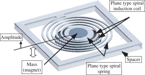
Figure 3.4 Schematic of silicon spiral microspring generator

Some analytical models have been proposed to examine the vibration system movement [12, 13, 15, 16]. For example, in 1998 Amirtharajah and Chandrakasan developed a linearized model to determine the maximum power output of an electromagnetic vibration-based generator [12]. In 2000, Li et al. [13, 15] proposed a simple power generation model using a frequency domain approach to examine the effects of the governing parameters of an electrical power generation system. In 1998, Williams et al. [16] used only a differential equation to analyze a vibration system in a microelectric generator, but did not discuss magnetic field distributions. The authors of the current study [17] constructed a vibration-based electromagnetic generator consisting of a magnet with a central cylindrical cavity inside and a movable helical low-temperature co-fired ceramic (LTCC) microspring with a multilayer silver induction coil. A simple analytical model was developed to analyze the mechanical motion of the spring-mass system located in the cavity of the magnet.

3.2 Comparisons between MCTG and SMTG

Generally, there are two types of microgenerator structures: the magnetic core-type generator (MCTG) and sided magnet-type generator (SMTG). In an MCTG, the magnetic field is generated by the interaction of a magnetic core element and a magnet in the center hole; in an SMTG the magnetic field is generated by the microinduction coil on the sides of the magnetic element.

Table 3.1 lists the differences between the elements of a MCTG and a SMTG. Properties such as volume and the magnetic field generation source, the assembly concept and the inductor structure for MCTG and SMTG types also differ slightly.

Table 3.1 Elements of types of microgenerator: MCTG and SMTG

Specification	Micro generator types
	MCTG type	SMTG type
Magnet No.	2	2
Total magnet thickness (mm)	4	4
Magnet hole radius (mm)	8.6	—
Total micro inductor thickness (µm)	240	180
Induction coil cross-section area (width × thickness) (µm)	90 × 10	88 × 6.2
Resistor inside induction coil (Ω)	0.3	0.49
Outside resistor (Ω)	0.31	0.51
Inductor hole radius (mm)	1.3	—
Spacer thickness (mm)	—	3 (2 × 1.5)
Spacer hole radius (mm)	—	8.6
Magnetic core height (mm)	4	—
Magnetic core outer diameter (mm)	1.1	—
Vibration mass (mg)	27.6	16
Total volume (mm3)	424	718

3.2.1 Magnetic Core-Type Generator (MCTG)

The assembly schematic of a standard magnetic core-type microgenerator is shown in Figure 3.5. This MCTG includes an LTCC microinductor, a magnetic core element, a magnet module, an oscillation mass, and an attached adjustable resistor in which the magnet module is composed of two NdFeB magnets attached on the upper and lower surfaces of the LTCC microinductor. Each magnet is 2 mm thick, and a cylindrical hole with a radius of 8.6 mm is located at its center. This cylindrical hole accommodates adequate space for the microspring oscillation. Accordingly, the magnetic elements provide not only the magnetic field but also the supporting frame for mechanical oscillation; 2-mm-thick NdFeB magnets are the commonly used specification. Because NdFeB magnets are commercially available, they present an advantage for cost-reduced mass-production.

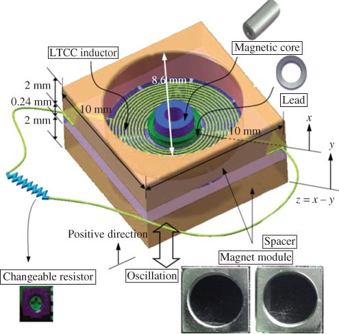
Figure 3.5 Assembly of a MCTG oscillation-type microgenerator [18]

A circular hole with a radius of 1.3 mm is at the center of the LTCC microinductor to create a vacuum leak inside, which results in the difficulty in the elements' fixtures. This problem can be resolved by using a microinductor with the same pattern to fix the elements; this is at the expense of increasing the manufacturing cost, however. The tubular magnetic core element has an inner and outer radii of 0.5 mm and 1.1 mm, respectively. It passes through the central hole of the microinducer and is located at central hole of the PM. Finally, a lead ring 27.6 mg in weight is used as the oscillation mass and is attached to the surface of the central ring structure of the inducer.

3.2.2 Sided Magnet-Type Generator (SMTG)

Figure 3.6 shows the assembly schematic of an SMTG which includes an LTCC inducer, a magnet module, two plastic spacers, an oscillation mass, and an attached changeable resistor.

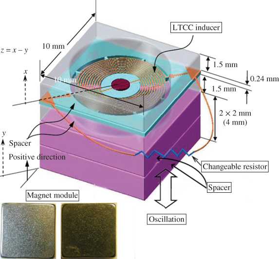
Figure 3.6 Assembly of a SMTG oscillation-type microgenerator [18]

3.3 Analysis of Electromagnetic Vibration-Induced Microgenerators

Analytical models of a microgenerator involve vibration-induced coupling issues of mechanical kinematics and electromagnetism. Some analytical derivations are developed to determine the relationship between these coupling issues. First, a formula is developed for vibrating kinematics. Based on Biot-Savart's law, the distribution of the electromagnetic spatial field is then established. Finally, according to Faraday's law, the behavior of electric inductance is predicted. The notation used in this model is summarized in Table 3.2.

Table 3.2 List of symbols, names, and units [18]

Symbol	Name	Unit
A	Cross-section area of microspring	µm2
	Radial unit vector	—
	Tangent unit vector	—
B	Magnetic field	T
Be	Effective magnetic field	T
	Time-varying effective magnetic field	T s–1
b	Loop radius of microspring	mm
Fs	Springing load force	N
I	Electric current	A
J	Second polar moment of microspring	µm4
k	Spring of stiffness	N m–1
ke	Equivalent spring of stiffness	N m–1
r	Turn radius of coil	—
Ts	Springing torsion	N m
t	Time	s
U	Springing strain energy	J
Y	Maximum amplitude	mm
y	Input excitation	mm
	Vibration amplitude	mm
	Vibration speed	mm s–1
Φ	Magnetic flux	WB
δ	Including angle	rad
(or EMF)	Electromotive force	V
i	Coil electromotive force	V
t	Total electromotive force	V
φ	Phase angle	rad
ω	Input frequency	rad s–1
ωn	Resonant frequency	rad s–1

3.3.1 Design of Electromagnetic Vibration-Induced Microgenerators

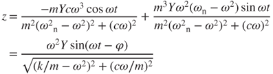
Figure 3.7a illustrates the configuration of a vibration-based electromagnetic micropower generator and its dimensions. Figure 3.7b shows a cross-sectional diagram, revealing the integration of the helical ceramic microspring and helical silver microcoil used to construct an inducer. Figure 3.7c shows a diagram of a single-layer inducer and design of the double supporting beam. The device shown in Figure 3.7a consists of two plastic spacers, a NdFeB PM and an LTCC inducer. The spacers are glued on the inducer to provide mechanical support and form a cylindrical cavity that is 8.6 mm in diameter and 1.5 mm deep, thereby providing sufficient space for vibration of the microspring. Each spacer is 1.5 mm thick. The NdFeB magnet has a residual induction (B_r) of 1.46 T. A system with double magnets has also been designed. The double magnet system has a total thickness of 4 mm, whereas the system with a single magnet is 2 mm thick. The entire volume of the meso-generator with double magnets is 10 mm × 10 mm × 7.18 mm (718 mm³). The oscillating mass of the center plate for the vibration is 16 mg. The mentioned cavity is of sufficient depth to accommodate the maximum vibration amplitude of the microspring.

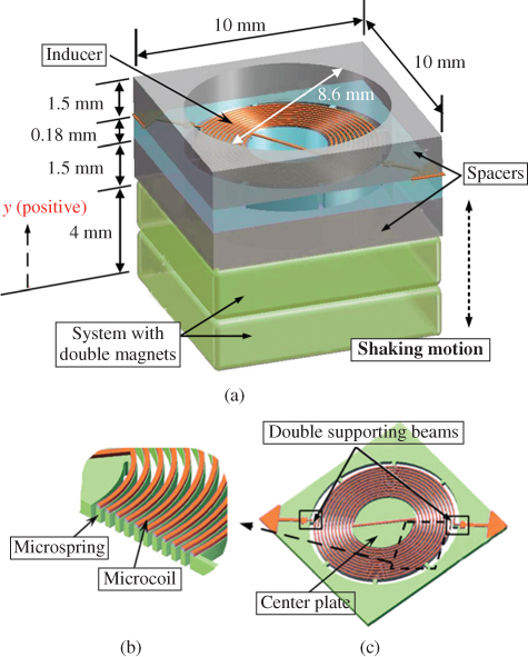
Figure 3.7 Design of vibration-based electromagnetic power generator: (a) configuration and the dimensions, (b) diagram of the cross-section, showing the integrated microspring and microcoil, and (c) diagram of single-layer inducer and design of the double supporting beam [18]

3.3.2 Analysis Mode of the Microvibration Structure

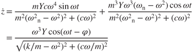
Figure 3.8 shows a schematic of a vibration-induced generator; Figure 3.8a depicts the operating kinematics, Figure 3.8b the supporting beam of the microspring and its geometric parameters, and Figure 3.8c configuration of the spiral microspring. The vibration system is composed of a seismic mass m, a spring stiffness k, and a damping coefficient c. When the rigid housing is moved with an input excitation y, the inertia mass has a relative motion z to the housing. The magnetic movement relative to the induction coil causes variations in magnetic fields and can then drive the conversion of mechanical energy to electric energy. The kinematics of the generator is described as

3.1

where is the vibration velocity. The input excitation is assumed to be a sinusoidal function expressed as

3.2

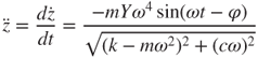
where Y is the excitation amplitude, ω is frequency, and t is time. The second-order differential of the input excitation with respect to time is

3.3

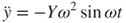
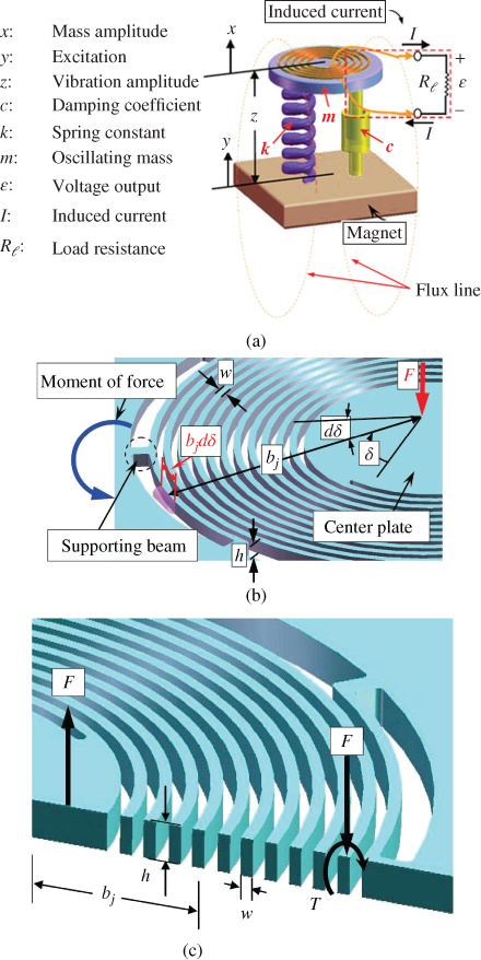
Figure 3.8 Illustration of the meso-generator: (a) in operating kinematics, (b) supporting beam of the microspring and its geometric parameters, and (c) configuration of the spiral microspring [18]

Substituting Equation (3.3) into Equation (3.1) yields

3.4

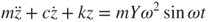
The solution to the second-order ordinary differential Equation (3.4) can be obtained analytically. The general expressions for the vibration position z and vibration velocity in the steady state are:

3.5

3.6

3.7

where 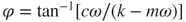is the phase angle and is the natural resonant frequency. In addition, the damping coefficient c can be obtained by measuring the vibration position z and velocity .

The springing strain energy U for one loop microspring-vibration system is composed of two terms from the spring torsion T_s and the applied force F_s, defined:

3.8

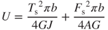
3.9

3.10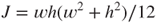

3.11

where G, J, and A are the silicon shear module, second polar moment of the microspring, and cross-section area of the microspring, respectively. The variables w and h are the width and the thickness of the microspring, respectively, and b is the radius of the microspring. Castigliano's theorem [18] indicates that the maximum displacement d is the partial derivative of springing strain energy U of Equation (3.8) with respect to the applied force F_s; that is,

3.12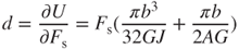

Hooke's law states that the spring stiffness k is the ratio of the applied force F_s to the maximum displacement d, as given by using

3.13

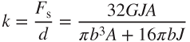
Substituting 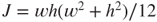and into Equation (3.13), the spring stiffness of a microspring with one single loop can be expressed:

3.14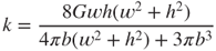

For an n-loop spring vibration system in the device, the equivalent spring stiffness k_e can be obtained using

3.15

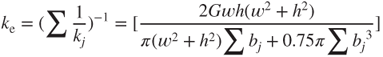
where b_j is the radius of the jth loop microspring.

3.3.3 Analysis Mode of Magnetic Field

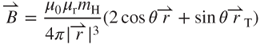
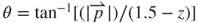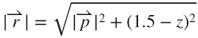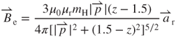
The behavior of a spatial magnetic field is described according to the relative position vector from the magnet to the induction coil and the tangent vector at the induction coil position in the spherical coordinate system, as shown in Figure 3.9a. Based on the image shown in Figure 3.9a, the geometric parameters of θ and can be expressed as and . Symbol represents the projected radial vector of the induction coil. The spacer thickness is 1.5 mm. When the magnet moves away from the induction coil, the magnetic field density around the induction coil becomes low. The magnitude of decays with the cubic of the distance, and is expressed regarding vacuum permeability μ₀, relative permeability μ_r, and the magnetic dipole of magnet m_H. From Biot-Savart's law [19], we obtain

3.16

3.17

3.18

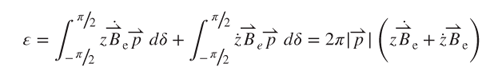
where θ is the inclination angle from the induction coil to the central symmetrical axis. Faraday's law of electromagnetism can predict the induced voltage output. Because symmetrical is evidently independent of the circumferential angle δ, a value of −π/2 to π/2 of δ is assumed (shown in Figure 3.9a) to simplify the analysis of . According to this law, the inducible electromotive force (EMF) is equal to the rate of the change of the flux while the magnetic field line is passing through an enclosed area vector (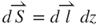) formed by an induction coil of an infinitesimal circle arc length () and a magnetic displacement dz. The inducible (EMF) is obtained using

3.19

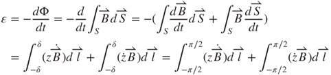
where Φ is the magnetic flux and is the enclosed area vector.

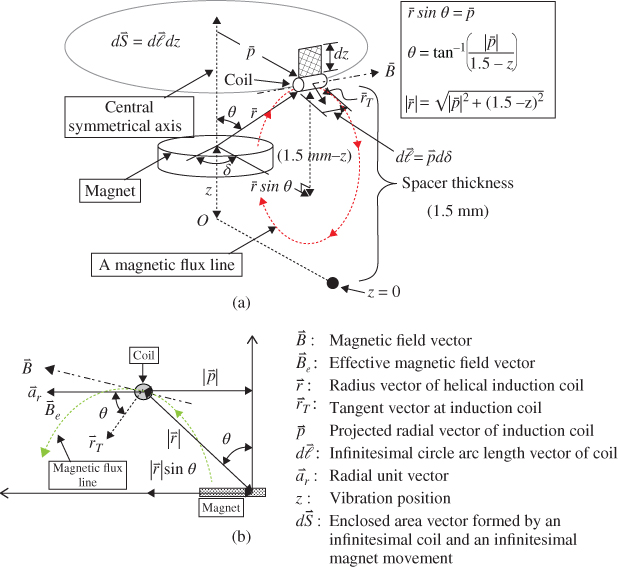
Figure 3.9 Schematic of (a) a three-dimensional magnetic field in the spherical coordination system (R, δ, θ) and (b) effective magnetic field [18]

Based on terms and in Equation (3.19), only the component of perpendicular to the vibration direction of the magnet contributes to the EMF. The effective magnetic field shown in Figure 3.9b can be derived as

3.20

or

3.21

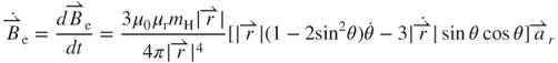
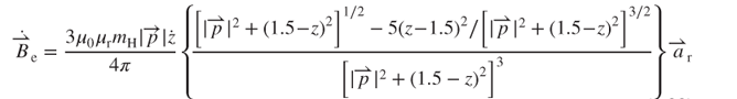
where is the radial unit vector. The effective magnetic field rate that is perpendicular to the vibration direction of the magnet can be obtained using

3.22

or

3.23

By substituting Equations (3.20) and (3.22) into Equation (3.19), the EMF for a single-turn induction coil can be rewritten as

3.24

The variable _i represents the EMFs on an induction coil of the ith turn. For a multiturn induction coil, the EMF for the ith turn is derived by substituting Equations (3.21) and (3.23) into Equation (3.24) to yield:

3.25

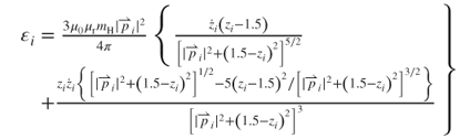
Based on Equation (3.25), the term of _i can be predicted by m_H, μ₀, μ_r, , z (Equation (3.5)), and (Equation (3.6)). The EMF on all of the induction coils is the sum of in the device, and can be written:

3.26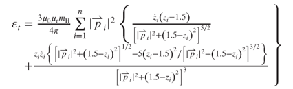

If an electric resistance R is linked with the induction coil, the induced current can be obtained using

3.27

The external resistance R is much larger than that inside the copper induction coil. For a sinusoidal EMF, the average power generation is expressed:

3.28

where the subscript rms denotes the root-mean-square value.

3.3.4 Evaluation of Various Parameters of Power Output

According to Equation 3.15, the equivalent spring stiffness k_e decreases non-linearly with the sum of the loop numbers. As shown in Figure 3.10, the curve of k_e exhibits a negative slope. Using a device with 12 loops as an example, the value of k_e is 5.05 N m^–1, in which the dimensions are 100 µm in width and 100 µm in interspace, the innermost loop radius is 1.7 mm and the minimum feature size is 40 µm in depth.

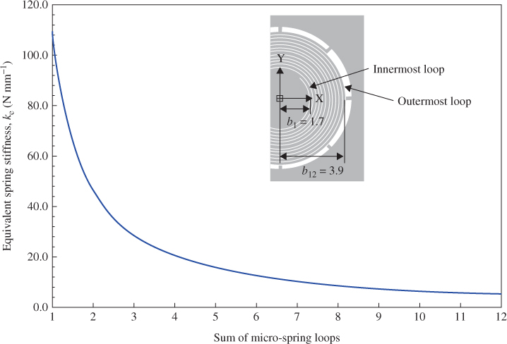
Figure 3.10 Graph of equivalent spring stiffness as a function of loop number of the microspring, microspring radius b₁ = 1.7 mm, b_J+1 = b_j + 200 µm, microspring width w = 100 µm, and microspring thickness h = 40 µm [18]

The magnetic field varies non-linearly with the position when the PM moves up and down. The simulated result based on Equation (3.16) is shown in Figure 3.11. The permeability μ₀ and relative permeability μ_r of copper induction coils are 4π × 10⁻⁷ H m^–1 and 0.9999, respectively. The graph indicates that the maximum value of is 0.314 T at the innermost turn of = 0.8 mm when the vibration position z is 1.5 mm. The direction of z is illustrated in Figure 3.7. The positive vibration direction points toward the induction coil, meaning that the distance between the PM and induction coil is reduced. A higher value of was found when the PM was closer to the induction coil. The minimum appears at the outermost turn of = 3.8 mm and approaches a constant value of 0.01 T, demonstrating that the magnetic field is inversely proportional to the distance between the magnet and induction coil, as indicated in Equation (3.16).

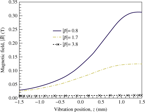
Figure 3.11 Analytical magnetic field on each induction coil of three unequal radii against vibration position [18]

Figure 3.12a,b depicts plots of the curve of the effective magnetic field and the effective magnetic field rate versus vibration position z, respectively, on each copper induction coil of three unequal radii . In Figure 3.12a, the magnetic field curve of is obtained from Equation (3.21). A maximum value was observed at each curve. The maximum value of for = 0.8 mm of approximately 0.201 T occurred at z = 0.96 mm, which can be obtained by setting the differential of Equation (3.21) to zero. The positions for the maximum magnetic field vary with the induction coil because of the non-linear magnetic flux lines (Figure 3.7). For instance, the for = 0.8 mm reduces to a minimum beyond z = 0.96 mm which is equal to y = −0.54 mm for a net distance of 0.54 mm and θ of π/4. This net difference between y and z is caused by the existence of vibrating-damping effects. In addition, a smaller is found at z of –1.5 and 1.5 mm, respectively. The value of is close to a constant of 0.005 T for equal to 3.8 mm.

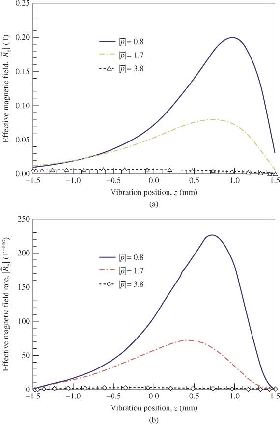
Figure 3.12 (a) Analytical effective magnetic field and (b) analytical effective magnetic field rate on each induction coil of three unequal radii against vibration position [18]

In Figure 3.12b, according to Equation (3.23) the largest value of is generated when the PM is at the positive vibration position z closest to the induction coil. The appearance of curves shows positive and then negative slopes with respect to z, in which the reason for the curvatures is as the case. For example, the maximum at z of 0.72 mm is 227.8 T s^–1 for equal to 0.8 mm. Values close to zero are found at z of −1.5 mm and z of 1.5 mm for each turn of the induction coil, respectively.

Based on Equations (3.5), (3.21), and (3.23), the relationship between and for equal to 0.8 mm, with respect to vibration position z, is obtained as shown in Figure 3.13. Both curves of and show a positive slope at a smaller value of z, which increases gradually according to z, and show an intersection at z of 0.8 mm corresponding to of 0.2 T and of 0.2 kT s^–1. Based on Equation (3.24), Figure 3.13 shows that the maximum value of EMF _i of the ith turn induction coil of approximately 2.02 mV is obtained at the intersection (z = 0.8 mm). The value of 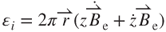is zero because = 0 and = 0 at the vibration position z of 1.5 mm.

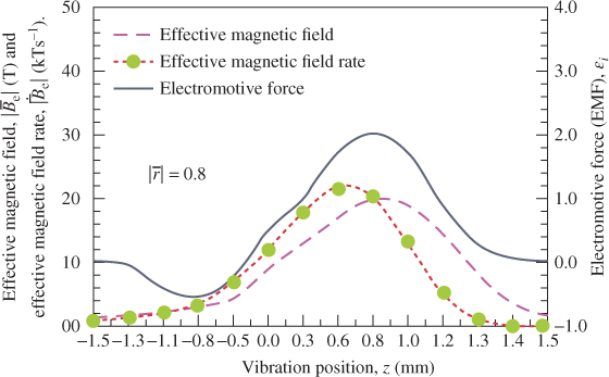
Figure 3.13 Comparisons between effective magnetic field, effective magnetic field rate and EMF with respect to vibration position [18]

Figure 3.14 shows the analytical value of the EMF _i from Equation (3.25) on each induction coil as a function of input excitation y (y = z − 1.5). The curves show that the highest value of _i is 2.02 mV for of 0.8 mm at y of –0.7 mm (z = 0.8 mm). This result agrees with that shown in Figure 3.13. The graph also indicates the variation of _i on each induction coil. Furthermore, for a larger , the generator exhibits a smaller _i. When y reaches –1.5 or 1.5 mm, the value of _i on each induction coil is approximately zero because = 0 and = 0.

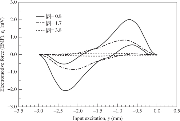
Figure 3.14 Analytical EMF of each induction coil of three unequal radii against input excitation; Y = 1 mm, ω_n = 120π rad s^–1, and y = z – 1.5 [18]

3.4 Analytical Results and Discussion

If the microspring is composed of two sets of springs (one clockwise or cw and the other counterclockwise or ccw), then the spring constant of this combined structure can be expressed as

3.29

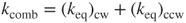
According to Equation (3.29), the relationship between the spring constant and the loop number is shown in Figure 3.15. Clearly, the spring constant decreases with increasing the loop number.

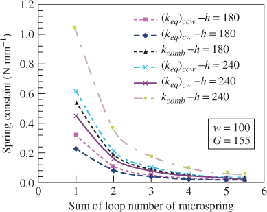
Figure 3.15 Relationship between the spring constant and the loop number [18]

For example, a combined spring with two loops is designed. The inner and outer radii of the spiral are 1.7 and 3.9 mm, respectively. The thickness, width, and gap of the elastic beam are 240, 90, and 400 µm, respectively. The combined spring constant () is 252 N m^–1. Under the same dimensional conditions, for a spiral number of 5.5 becomes 38.5 N m^–1. Accordingly, , , and have the same tendency. The spring constant increases as the spiral radius b and loop number decrease. For example, = 298 N m^–1 for b = 1.9 mm is smaller than = 417 N m^–1 for b = 1.7 mm.

After rearranging Equation (3.20), the resonance frequency ω_n can be expressed

3.30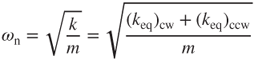

or

3.31

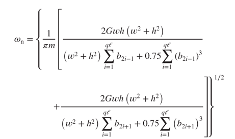
According to Equation (3.31), the effects of spring beam width w and thickness h on the resonance frequency ω_n are shown in Figure 3.16. It is known that, as the width w increases from 50 to 150 µm and 180 µm < h < 240 µm, ω_n increases with w and h. This result indicates that the resonance frequency of the spring structure is affected by the spring beam width and thickness.

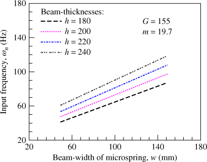
Figure 3.16 Effects of spring beam width w and thickness h on the resonance frequency ω_n [18]

3.4.1 Analysis of Bending Stress within the Supporting Beam of the Spiral Microspring

During system oscillation, the spiral microspring supports the oscillation structure. The bending moment on the surface of the supporting beam, which results in a bending stress, is shown in Figure 3.17. The differential bending moment dM results from a force F and a differential length dl, that is,

3.32

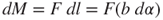
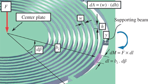
Figure 3.17 Schematic of force and bending moment on the supporting beam [18]

Integrating Equation (3.32) along one loop yields the total bending moment on one loop of the spiral spring.

A microspring is a structure of many loops. Thus, the total bending moments on the entire spiral spring are

3.33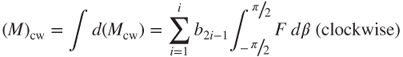

and

3.34

where F is the force resulting from acceleration and mass (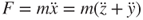). The maximum moments occurring at the maximum amplitude are

3.35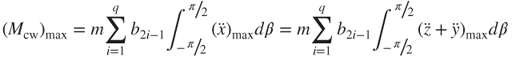

and

3.36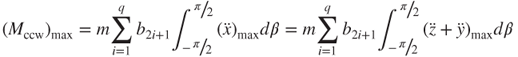

where acceleration and can be obtained from Equations (3.7) and (3.3), respectively.

Figure 3.18 shows the configuration of the supporting beam at a bending moment. The supporting beam bending upwards denotes positive moment, as shown in the figure. Cross-section a–a is parallel to cross-section c–c before bending, whereas sections a–a and c–c form an angle dθ after the bending moment.

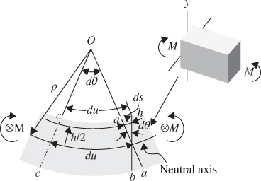
Figure 3.18 Configuration of the supporting beam under a bending moment [18]

If the curvature radius of the neutral axis is ρ, the curve length du for the neutral axis with angle dθ is

3.37

and

3.38

The strain is defined as the ratio of the displacement ds to the original length du, that is,

3.39

Substituting Equation (3.38) into Equation (3.39) yields

3.40

According to the material mechanics definition, stress is the product of elastic modulus and strain; that is, and the stress σ on the cross-section of the supporting beam can be determined via

3.41

where the minus sign denotes a compressive stress. Based on the equilibrium force, the imposed moment must be equal to that resulting from the internal stress, that is,

3.42

where dA (= w dh) is the infinitesimal cross-sectional area of the beam. Combining Equations (3.41) and (3.42) yields

3.43

where I_b is the cross-sectional area moment inertia, defined

3.44

Equation (3.44) indicates that the bending stress σ is proportional to the bending moment M, and that the maximum stress σ_max occurs on the surface of the beam (with the maximum value of h). Combining Equations (3.43) and (3.41) yields the maximum stress, defined:

3.45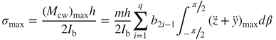

or

3.46

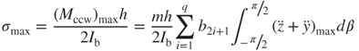
where and are functions of the maximum amplitude Y, frequency ω and time t. Based on Equation (3.46), aside from the oscillation parameters , , and m, the maximum bending stress is also affected by the spiral microspring geometric parameters such as thickness h, width w, spiral radius b and loop number j. If the maximum stress is smaller than the material strength, the spring structure would be safe. The maximum stress can therefore be used as one of the criteria of the optimal structural design.

The effects of the beam width w and the maximum amplitude Y on the maximum bending stress σ_max are shown in Figure 3.19. The beam thickness is h = 240 µm.

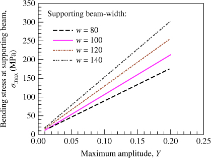
Figure 3.19 Effects of maximum amplitude on the maximum bending stress [18]

3.4.2 Finite Element Models for Magnetic Density Distribution

The commercial finite element software Ansoft Maxwell is used to analyze the magnetic field distribution inside a MCTG. An analytical model is proposed to analyze the magnetic field distribution inside a SMTG.

As shown in Figure 3.7, a space exists between the magnetic core element and the PM in a MCTG. The spiral microinduction coils oscillate inside the space, where an effective magnetic field exists. Finite element simulations can be used to observe the magnetic field distribution in the space. When the effective magnetic field is orthogonal to the movement of the induction coils, a larger induced EMF can be obtained. Ansoft Maxwell is commonly used finite-element software, which has strong pre- and post-processing abilities. The magnetic field distribution can be easily illustrated. To understand the effects of the magnetic thickness and magnetic core materials on the magnetic field, NdFeB and nickel-zinc-iron (NiZn) are used as the core materials and the magnetic thicknesses are 4 and 5 mm. NdFeB is a type of hard magnetic material. Compared to other PMs, it exhibits magnetic properties that are more favorable, such as the maximum magnetic energy product. In addition, NdFeB offers high magnetic density even under a small size or shape. NiZn is a type of soft magnetic material. Because NiZn has the properties of low assembly cost and low eddy current loss, it is widely used and a potential magnetic material. The residual induction B_r densities for NdFeB and NiZn are 1.46 and 0.17 T, respectively. Table 3.3 summarizes the other magnetic properties.

Table 3.3 Physical magnetic properties of NdFeB and NiZn (measuring temperature is 25 °C) [18]

	Residual induction Br (T)	Maximum energy product BH,max (kJ m–3)	Coercive force Hcb (kA m–1)	Intrinsic coercive force Hcj (kA m–1)
NdFeB	1.457	417.2	955.5	1009
NiZn	0.17	26.26	0.05	0.06

Figures 3.20–3.23 show the simulation results with different magnetic thicknesses and core materials. Figures 3.20 and 3.21 show the results without using magnetic core materials and using magnets with thicknesses of 5 mm and 4 mm. In the figures, the maximum magnetic field densities are B = 0.83 and 0.82 T for Figures 3.20 and 3.21, respectively. The maximum magnetic field occurs near the upper and lower surfaces of the magnet. Because the position corresponding to the maximum magnetic field is not inside the extent of the induction coils oscillation, the induced EMF cannot be increased.

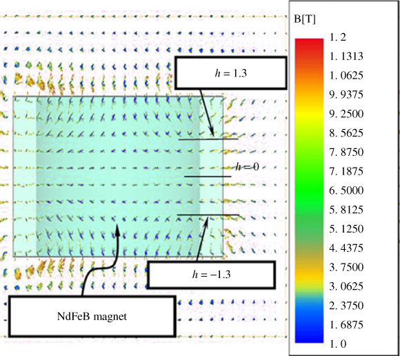
Figure 3.20 Simulation results for magnet thickness of 5 mm and without magnetic core materials [18]

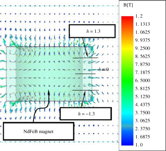
Figure 3.21 Simulation results for magnet thickness of 4 mm and without magnetic core materials [18]

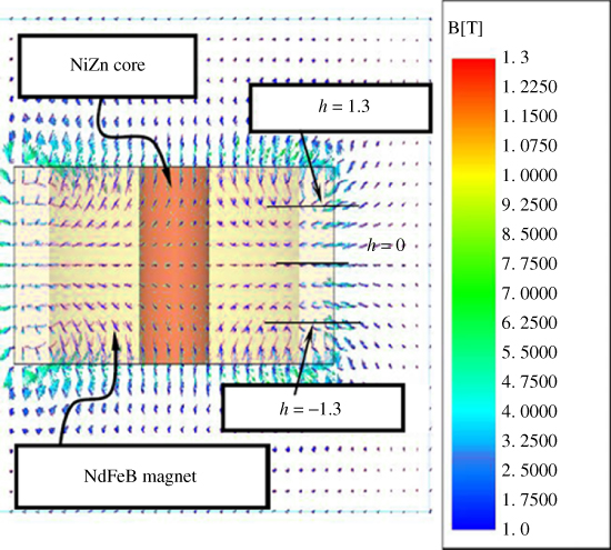
Figure 3.22 Simulation results for NiZn magnetic core material with magnet thickness of 4 mm [18]

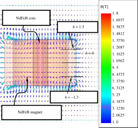
Figure 3.23 Simulation results for NdFeB magnetic core material with magnet thickness of 4 mm [18]

Nevertheless, as shown in Figures 3.20 and 3.21, a special zone is inside the central cylindrical space that offers an effective magnetic field. The extent of this special zone is along the thickness direction of the magnet (the same direction as that of the induction coil movement). Regarding the upper magnet (Figure 3.7), the effective magnetic field points outward from the magnetic core element. Accordingly, it is speculated that the induction coil movement direction is orthogonal to the effective field direction, and a maximum EMF can be generated. The simulation results also indicate that the effective field density approaches 0.3 T from z = 0 to 1.3 mm in the special zone. Conversely, regarding the lower magnet (Figure 3.7), the effective magnetic field points inward to the magnetic core element. The extent of the special zone is from z = 0 to –1.3 mm. The simulation results in Figures 3.20 and 3.21 illustrate that the effective magnetic density is not affected significantly by the positions of the thickness direction of the magnet, which implies that the effective magnetic field density variation rate can be regarded as zero. Based on the comparisons between Figures 3.20 and 3.21, the effects of the magnetic thickness on the magnetic density are quite small.

Figures 3.22 and 3.23 show the results of using a 4-mm-thick magnet and magnetic core materials of NiZn and NdFeB, respectively. The simulation results in Figures 3.22 and 3.23 illustrate that the patterns of the magnetic field are quite similar to those in Figures 3.20 and 3.21, and the maximum effective magnetic field densities are 0.35 T for the NiZn magnetic core and 0.46 T for the NdFeB magnetic core. These results imply that the NdFeB magnetic core is more effective than the NiZn magnetic core at increasing the effective magnetic field density.

3.4.3 Power Output Evaluation

Figure 3.24 shows the electron-shifting physical phenomenon as a conductor of an infinitesimal length dl moving with a velocity within a magnetic field B. As the conductor moves, the magnetic field forces the electron to move to one end of the conductor. Conversely, the opposite end of the conductor has positive electricity. At that moment, there is a voltage drop between the two ends and there is also a Coulomb attraction force between them. This separation situation continues until the magnetic force and electric force counteract with each other and a balance situation is achieved. In the procedure, the infinitesimal length dl with a movement dz constitutes an infinitesimal area variation dS. The magnetic flux Φ passing through this area dS is

3.47

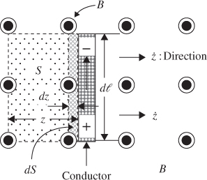
Figure 3.24 Electron shifting physical phenomenon as a conductor moving within a magnetic field [18]

According to Faraday's law of electromagnetic induction, the EMF is the magnetic flux variation rate passing through a conductor with an area variation dS, that is,

3.48

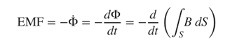
By applying the differentiable product rule, Equation (3.48) can be rewritten as

3.49

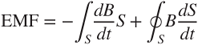
where the term dB/dt is the magnetic flux variation rate . The term dS/dt denotes the infinitesimal area variation rate , and is equal to the product of the infinitesimal length dl and moving velocity . Total area S is the product of dl and moving distance z. Equation (3.49) can therefore be rewritten as

3.50

Based on Equation (3.50), the magnitude of EMF is affected not only by the magnetic field B, the magnetic field rate , but also by the oscillation amplitude z, oscillation speed , and the conductor length l. According to the vector product in the second term, the EMF achieves the maximum because B and are orthogonal to each other.

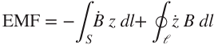
If the spiral coil shape is circular with a constant radius b (), the EMF for a single loop microconductor is

3.51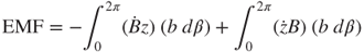

For a conductor coil with a multiloop structure, the EMF becomes

3.52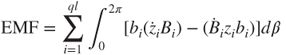

where ql denotes the loop number of the spiral spring. Figure 3.25 shows the top view of an LTCC microconductor adopted from Figures 3.1 and 3.2, which indicate two groups of spiral conductor coil structures (Coil_ABC and Coil_DEF). The first group Coil_ABC is clockwise (cw) from Point A to Point B and Point C. The second group Coil_DEF is counterclockwise (ccw) from Point D to Point E and Point F.

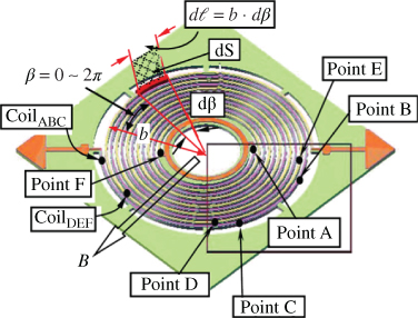
Figure 3.25 Configuration of two groups of spiral conduction coils within a spiral spring [18]

As the microconduction coils oscillate, the EMF_cw in group Coil_ABC generates along Point A to Point B and then to Point C:

3.53

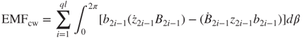
The induction current flows through Point A and Point B, and then to Point C. By contrast, the EMF_ccw in group Coil_DEF is

3.54

The induction current I_DEF in group Coil_DEF flows through Point D and Point E, and then to Point F. The total voltage of the EMF is obtained by adding Equations (3.53) and (3.54) (EMF = EMF_cw + EMF_ccw), and can be measured using an oscilloscope.

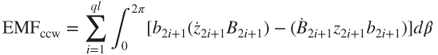
Figure 3.26 shows the relationship of the total induced voltage and the coil movement direction . As the path moves from Position 1 to Position 2 and then to Position 3, the induction voltage in the microinduction coils is positive. However, as the path moves from Position 4 to Position 1 and then to Position 2 (the lowest position to the highest position during the oscillation), the induced voltage is negative. The maximum induced voltage occurs at Position 2. The results are consistent with those obtained according to the previously stated magnetic field variation rate (Figure 3.22). These results also verify the validity of using the model with the magnetic field variation rate.

Figure 3.26 Relation of induced voltage to oscillation position and speed [18]

Figure 3.27 depicts the current flow direction in the two coil groups, Coil_ABC and Coil_DEF. The coils move from the top position to the bottom position (negative velocity). In the figure, the direction of I_ABC is opposite to that of I_DEF, because the voltage drop of EMF_cw is different from that of EMF_ccw. The EMF is affected by magnetic field B, magnetic field rate , amplitude z, oscillation speed , and coil length l. Comparing the difference between Equations (3.53) and (3.54), the total current is I_total = I_ABC + I_DEF. However, because the oscillation velocity is positive (from the bottom position to the top position), the current flow directions are opposite to those in Figure 3.27.

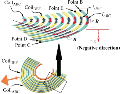
Figure 3.27 Schematic of current direction and induction coil oscillation [18]

Because of the effect of the material properties and internal structure, the microinduction coils intrinsically produce a resistance-inductance (RL) effect. Figure 3.28 shows the equivalent electric circuit of a microgenerator system, where R_l denotes the changeable resistor attached from outside. and denote the internal resistance and inductance of the microinduction coils, respectively. As it is attached, a current output can be obtained.

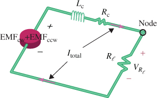
Figure 3.28 Equivalent electric circuit of a microgenerator [18

According to Kirchhoff's voltage law, the sum of the voltage that drops across every element around a closed loop is zero. Thus, at the node in Figure 3.15, the sum of the voltage that drops at EMF, , R_l, and is zero, that is,

3.55

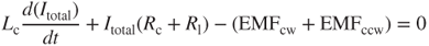
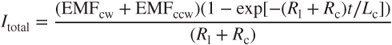
The solution of the output current I in Equation (3.55) can be expressed as

3.56

The flow direction of the current is determined according to Fleming's right-hand rule, as shown in Figure 3.29, in which the directions of the forefinger, thumb, and middle finger denote the directions of the magnetic field, inductor movement, and current flow, respectively. They are orthogonal to one another. Because a current I_total flows through the circuit and a voltmeter is connected to the both ends of the changeable resistor R_l, an induced voltage can be measured, the value of which is

3.57

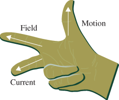
Figure 3.29 Fleming's right-hand rule

Substituting Equation (3.56) into Equation (3.57) and rearranging yields

3.58

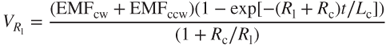
Based on Equation (3.58), the voltage is a function of time. When time t is large, the term 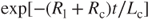approaches zero and the steady state of the voltage response is

3.59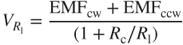

Because , the maximum value of can be obtained for the microgenerator.

If the microinduction coils are implemented into the multilayer parallel structure with the same node, and the resistance of each layer is assumed to be the same for R, then the resistor for each layer could be regarded as a parallel circuit and the total equivalent resistance R_c could be obtained using

3.60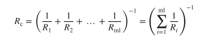

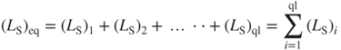
where the subscript ml denotes the number of microinduction coil layers. As the current flows through the circuit, an electromagnetic coupling action occurs, resulting in an inductance effect. Two sources result in this current-induced inductance effect. The first is called ‘intergap inductance’ and the second is ‘interlayer inductance’. Intergap inductance L_S can be regarded as a series circuit, and the equivalent intergap resistance (L_S)_eq can be calculated via

3.61

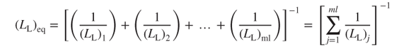
The other inductance effect occurs at the interlayers. The interlayer inductance L_L can be regarded as a parallel circuit and the equivalent interlayer resistance (L_L)_eq be calculated via

3.62

where ml denotes the number of layers of the microinduction coils. Using electric circuit formulas, the whole equivalent inductance L_c can be obtained by incorporating Equations (3.61) and (3.62):

3.63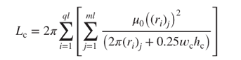

where μ₀, w_c, and h_c denote the magnetic-conductance coefficient (4π × 10⁻⁷ H m^–1), and the width and thickness of the induction coils, respectively.

Based on electric circuit theory, in an electric system the average power output P_avg is a function of the attached resistor R_l and the root-mean-square voltage output is , as expressed below:

3.64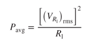

3.65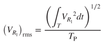

where T_P is the steady-state oscillation period. Equation (3.67) indicates that P_avg decreases with an increase in R_l. The maximum occurs for ; however, P_avg is not necessarily the maximum value. PD is defined as the ratio of the average power output P_avg to the device volume V, that is,

3.66

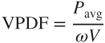
Clearly, a microgenerator can have a relatively high PD. The characteristics of a microgenerator can also be evaluated according to volumetric power density per frequency (VPDF) or mass power density per frequency (MPDF). VPDF is defined as the ratio of the average power output P_avg to the product of device volume V and frequency ω, that is,

3.67

MPDF is defined as the ratio of the average power output P_avg to the product of oscillation mass m and frequency ω, that is,

3.68

Clearly, a microgenerator can have a relatively high VPDF or MPDF if the volume or mass is quite small.

3.5 Fabrication of Microcoil for Microgenerator

3.5.1 Microspring and Induction Coil

Figure 3.30a illustrates the key processes of the LTCC inducer. In Step 1, a printer (Hotshine Corp. 2000 model manufactured in Taiwan) prints silver paste onto the green sheet by using a screen-stencil with a coil pattern. The pattern with a 10-µm-thick emulsion is fabricated using standard photolithography techniques. After the printing procedure is complete, both the silver paste and the PET tape on each green sheet is oven-dried at 80 °C for 30 min. In Step 2, a carbon-dioxide (CO₂) laser driller (Sumitomo GSD 1400TW model) is employed to fabricate an interspace between coils. A helical microspring of 5.5 unequal radius loops and a center circle plate are formed by laser cutting. Each layer is fabricated on green tape by repeating these steps. In Step 3, the green tape is reversed with the PET facing upward. A rubber roller (Hotshine 200FA model) is used to strip the PET tape from the green sheet and a vacuum holder catches the residual ceramic film.

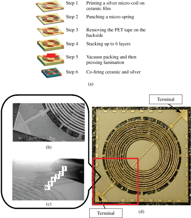
Figure 3.30 A sintered inducer: (a) illustration of LTCC fabrication, (b) observation of the six-layer coils via X-ray fluoroscopy method, (c) SEM image of the supporting beams and its terminal, and (d) photograph of appearance [18]

In Step 4, the vacuum holder stacks layers of film with an alignment accuracy of c. 18 µm, which places a limit on the total number of layers. For example, in the six-layer film stack, a stacking error of 108 µm is acceptable because it is smaller than the unfired microspring interspace of 116 µm. The vacuum packing in Step 5 protects the green structure and eliminates remaining bubbles. The films are laminated using an isotropic high press of 20.6 MPa in a pressing machine (ABB Corp. IL102010-SS model in USA) and liquid water is used as a medium. The films can be pre-adhered to each other after being maintained at 75 °C for 30 min. Using silver paste, two electrodes are painted over the two terminations of each coil and dried at 100 °C for 10 min.

In Step 6, the green material is hardened in a high-temperature furnace (UF Corp. K4U model manufactured in Taiwan). LTCC multilayer structures consist of different materials such as ceramic and silver, which are co-fired in one step. Sintering promoters play an essential role in the adhesion strength between the silver coil and the ceramic microspring. The LTCC co-firing fabrication allows for processing in ambient air without chemical oxidization. The heating profile is divided into two stages. The first is heating at 350 °C for 2 h. At this stage, the organic binder in the ceramic slurry is burnt away, leaving behind voids in the structure. The second stage involves sintering the materials and allows for the formation of covalent bonds. The temperature is ramped at 0.16 °C s^–1 from room temperature and heats at 850 °C for 30 min. During the sintering process, the voids left by the released binder are filled with ceramic and glass and the entire volume of the inducer becomes dense. The resulting shrinkage values of the in-plane and in-thickness dimensions are 0.16 and 33.3%, respectively. The difference in the shrinkage values can be attributed to the anisotropic surface area. After this sintering step, an inducer with a helical-multilayer structure consisting of a ceramic microspring and silver microcoil is constructed.

The six-layer coils in the ceramic structure as seen using an X-ray fluoroscopy method are shown in Figure 3.30b. Figure 3.30c shows a scanning electron microscope (SEM) image of the microspring. The process of multilayer LTCC fabrication enables the inducer to be constructed. Coils in the different layers are connected at the terminals. Figure 3.30d shows a photograph of the sintered inducer. The sintered microspring has a beam thickness of 180 µm, a beam width of 100 µm, and a beam interspace of 100 µm. The resulting structure has a 1.7 mm innermost helical loop radius, and a 3.9 mm outermost helical loop radius. The cross-sectional area of sintered microcoil is 90 µm (line width) × 10 µm (line thickness). Table 3.4 lists all of the material properties and geometric parameters.

Table 3.4 Copper and permanent magnet material properties and geometric parameters [18]

Symbol	Name	Constant	Unit
c	Damping coefficient	3 × 10−8	kg m s
G	Silicon shear modulus	66.7	MPa
h	Thickness of microspring	40	µm
m	Seismic mass	8.35 × 10−7	kg
mH	Magnetic dipole	6.13 × 10−3	A m2
R	Copper resistance	16	Ω
w	Width of microspring	100	µm
μ0	Copper permeability	4π × 10−7	H m–1
μr	Copper relative permeability	0.9999	—
σc	Copper conductivity	5.8 × 10−7	Ω m−1

3.5.2 Microspring and Magnet

A microspring with a helical beam and a center plate was fabricated. The key techniques were DRIE, co-sputtering, and reactive ion etching (RIE), as schematically illustrated in Figure 3.31a. In Step 1, a silicon wafer is selected to fabricate the microspring structure using DRIE. In Step 2, a ferro-platinum (FePt) PM membrane is co-sputtered on the center plate. For the PM used in this study, a magnetic dipole m_H of 6.13 × 10⁻³ A m² can be achieved after annealing. In Steps 3–6, a silicon nitride (Si₃N₄) layer and etching mask are used to remove the back side of the wafer via RIE (refer to [20] for additional details). Figure 3.31b shows an SEM photo of the microspring structure.

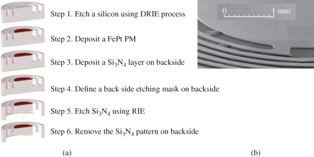
Figure 3.31 (a) Fabrication processes for microspring and FePt by DRIE method. (b) SEM photo of the microspring [18]

According to Equation (3.15), the non-linear equivalent spring stiffness k_e decreases with the loop number. As shown in Figure 3.13, the curve of k_e exhibits a negative slope. Considering a device with 12 loops, for example, the value of k_e is 5.05 N m^–1, in which the dimensions are 100 µm in width and 100 µm in interspace, and the innermost loop radius is 1.7 mm and the minimum feature size is 40 µm in depth. The value of k_e for the single loop spring is 108 N m^–1.

The material of the inducer before fabrication consists of green sheets (Heraeus HL2000) and silver paste (Heraeus TC0308). The dimensions of each green sheet are 150 mm × 150 mm in surface area and a thickness of 95 µm. The ceramic slurry is mixed with the aluminum oxide (Al₂O₃) powder, the glass powder, and binder powder in proportion. The soft, pliable, and abraded characteristics of green tape are beneficial to laser cutting. Laser cutting involves fabricating various shapes and special structures for MEMS. Furthermore, by using the silver material with favorable conductivity and a multilayer structure, the LTCC technique allows for inducer fabrication that benefits the current output induced in the energy conversion processes.

3.6 Tests and Experiments

3.6.1 Measurement System

After fabricating the meso-generator, several measurements were made to characterize the performance of the device. Figure 3.32 shows the block diagram of the measurement set-up and the photograph of the experimental instruments. As shown in the graph, a sinusoidal waveform of input amplitude and input frequency were derived from an arbitrary waveform generator (Agilent 33220A model). A power amplifier (Data Physic 100 W model) was used to magnify the signal from the waveform generator, allowing it to control a shaker (Data Physic PA100E) that provides the mechanical vibration input. An accelerometer (PCB 357B61 model) was attached to the top platform of the shaker to measure the vibration acceleration. Table 3.4 lists the material properties and geometric parameters used in analysis.

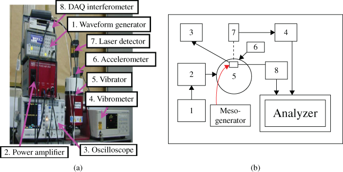
Figure 3.32 Measurement set-up: (a) block diagram and (b) photograph of the experimental instruments [18]

The meso-generator was fixed on the top of the accelerometer. An interferometer of data acquisition (DAQ) was used between the accelerometer and the analyzer to collect vibration-acceleration data. The shaking motion passes through the housing of the meso-generator, into the microinducer. A laser displacement vibrometer (Keyence LC-2401 model) with a laser detector was used to measure the mechanical vibration displacement. Finally, a variable resistor was connected directly to the terminals of the inducer. When the induced current passes through the variable resistor during vibration, a digital storage oscilloscope (GW Instek GDS-2062 model) measures both the induced voltage output and the induced current output from the meso-generator. In addition, the viscous damping coefficient can be measured by removing the variable resistor.

3.6.2 Measurement Results and Discussion

After measurement, a spring constant of k = 29.4 N m^–1 for 0.58 g (g = 9.8 m s^–2) of input vibration acceleration was obtained for the system at natural vibration frequency ω_n = 69 Hz and maximum amplitude of Y = 0.03 mm. In addition to the suitable operating parameters in the system, to investigate the effects of number of coil layers and number of magnets on voltage and current output, four samples were made. Only one magnet was designed in Samples 1, 2, and 3, whereas two magnets were designed in Sample 4. In Samples 1, 2, 3, and 4, there were 1, 2, 6, and 6 layers of induction coil, respectively. The specifications and the measured coil resistances for the four samples are listed in Table 3.5.

Table 3.5 Specifications of all samples [18]

Structures	Sample number
	1	2	3	4
Number of magnet	1	1	1	2
Number of coil layer	1	2	6	6
Thickness of inducer (mm)	0.18	0.18	0.18	0.18
Thickness of single spacer (mm)	1.5	1.5	1.5	1.5
Thickness of magnet system (mm)	2	2	2	4
Entire volume of meso-generator (mm3)	518	518	518	718
Coil resistance (Ω)	2.96	1.45	0.49	0.49

Figure 3.33a,b show the induced voltage output and induced current output I versus time, respectively. As shown in Figure 3.33a, a maximum voltage output in excess of 37 mV was found for Sample 1. The voltage output curves for Samples 1, 2, and 3 are similar, because the layered coils are all connected at common terminals. However, the maximum voltage in Sample 4 is 44.5 mV, which is larger than those in Samples 1–3. In comparing Samples 3 and 4, the voltage output is more sensitive to a change in the number of magnets than the number of coil layers. The voltage output for Sample 4 (2-magnet system) is c. 1.2 times that of Samples 1–3 (1-magnet systems). This demonstrates that increasing the voltage output involves increasing the number of magnets.

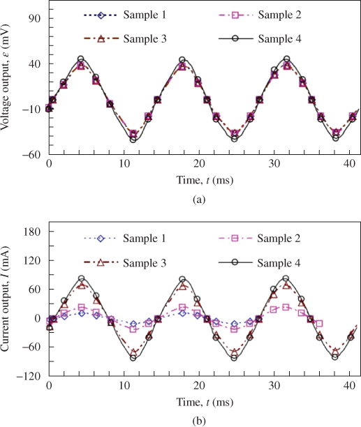
Figure 3.33 Results of electricity generation: (a) voltage output curve versus time and (b) current output curve versus time [18]

In Figure 3.33b, the induced current of Sample 3 is shown to be larger than that of Sample 1. The maximum induced current of 69 mA corresponding to Sample 3 is c. 5.95 times greater than the 11.6 mA value of Sample 1. Furthermore, the maximum current output of Sample 4 of 83.1 mA is c. 1.2 times greater than the output of Sample 3. This result reveals the special property of high-current and low-voltage output in this generator, which is similar to that found in Table 3.1 [8]. We also found that the increasing rate of induced current is proportional to both the number of coil layers and the number of magnets. The slope extracted from a plot of induced current versus time for Sample 4 is higher than the slope extracted from Sample 3 data, indicating that the influence of the number of magnets on the current output is larger than the number of coil layers. The maximum root-mean-square value of the measured current output induced in Sample 4 is I_rms = 56.4 mA.

In addition, Figure 3.34a and b depict the maximum average electrical power output versus number of coil layers and number of magnets, respectively. Figure 3.34a shows that the average power output in a multilayer coil system is higher than that in a single coil layer system, with the maximum P_avg increasing in proportion to the number of layers. For example, the maximum P_avg of 0.67 mW for Sample 3 (which has six layers) is approximately six times larger than the maximum P_avg of 0.11 mW for Sample 1 (which has one layer). Sample 2 has a maximum P_avg of 0.22 mW, twice as large as that of Sample 1. Figure 3.34b indicates an increasing value of maximum average power output with the number of magnets. The double magnet system in Sample 4 yields a larger value of maximum P_avg (1.56 mW) than the single magnet system in Sample 3 (0.67 mW). Our results indicate that the number of magnets is more important than the number of coil layers, as was the case for the current output.

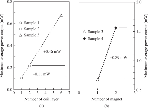
Figure 3.34 Measurements of electrical output: (a) maximum average power output versus number of coil layers for single magnet and (b) maximum average power output of six-layer coil versus number of magnets [18]

For such vibration-induced microsources, the energy-to-size ratio is a crucial criterion for determining when to evaluate the generator performance. The PD is a commonly cited criterion related to device volume, and is defined as the power output divided by the entire volume of the generator. Another parameter is the normalized power density (NPD), which is derived from the power output per square of input vibration acceleration. For example, Sample 4 has a higher PD of 2.17 µW mm^–3 than that of Sample 3, which is smaller only than the value of 2.2 µW mm^–3 [18]. Moreover, Sample 4 has a higher NPD of 6.46 µW mm^–3 g^–2 (g = 9.8 m s^–2) than that of Sample 3. Overall, results indicate that multiple magnets (high magnetic field) and a multilayer coil design can enhance the performance of a generator such as Sample 4. Measurements show that the meso-generator has a high power output because of the high current levels. Although the voltage output is sometimes as low as 44.5 mV, it can be increased to more reasonable levels by optimizing circuitry in the microsystem. Generators wired in series would have a much larger EMF than a single device.

3.6.3 Comparison between Measured Results and Analytical Values

Figure 3.35 shows the relationship of vibration amplitude z versus time. The orientation of vibration amplitude is shown in Figure 3.8a. This experiment is used to ensure that the distance swept out by the vibration is within the spacer thickness. Results confirm that the vibration ranges from vibration amplitude of z = 1.47 mm to z = 1.53 mm. The maximum amplitude of the coil is close to the maximum amplitude of the shaker, Y = 0.03 mm, because of the suitable spring constant. Because the oscillating mass is able to more completely sweep through the allowable space with a larger vibration acceleration and higher velocity, this implies that spring behavior in a generator increases the power output. In the same figure, the predicted vibration amplitude follows the same trend as measured result. The difference is 1.5%, possibly because of the predicted spring constant and damping coefficient.

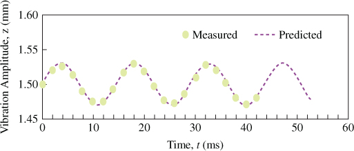
Figure 3.35 Experimental and predicted vibration amplitude versus time [18]

In Figure 3.36a,b, the peak points of the analytical and experimental values match favorably. However, the waveforms of the simulation results show different slopes at zero EMF and I. The reason for the curvatures possibly resulted from the simplifying model and the calculating error in the non-linear effective magnetic field and effective magnetic field rate. This indicates that the effective magnetic field and magnetic field rate are more sensitive to a change in EMF and I output than other governing parameters such as vibration position and velocity in this case.

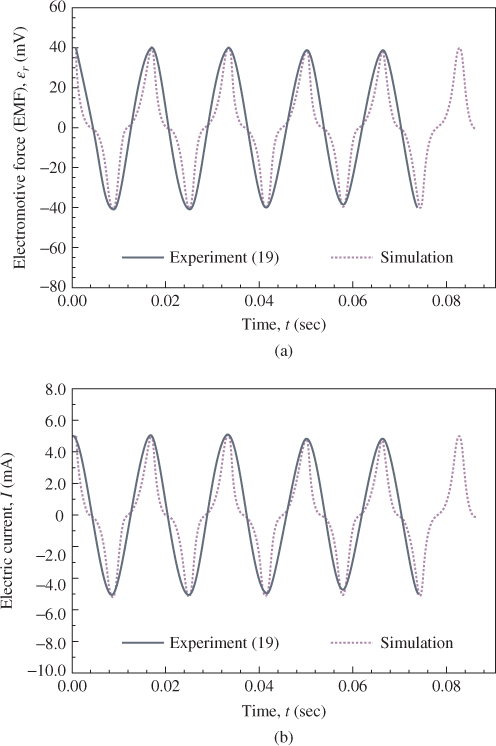
Figure 3.36 Comparisons between analytical and experimental EMF and electric current against time: (a) electromotive force and (b) electric current. ω_n = 120π rad s^–1, Y = 1 mm, and R = 8Ω [18]

3.7 Conclusions

3.7.1 Analysis of Microgenerators and Vibration Mode and Simulation of the Magnetic Field

An analytical expression for the electrical outputs of a vibration-induced microgenerator associated with coupling issues of mechanical kinematics and electromagnetism was established based on Castigliano's theorem, Hooke's law, Biot-Savart's law, and Lenz's law. The analytical results showed that the equivalent spring stiffness k_e of the microspring decreased with the loop number. The analytical values of k_e for 12 loops and a single loop by using the proposed formula were 5.05 and 108 N m^–1, respectively. A higher magnetic field around the induction coils was found, whereas the PM was close to the induction coil. The maximum is c. 0.314 T when the PM was closest to the induction coil. The values of the maximum effective magnetic field and effective magnetic field rate decreased with the projected radial distance of the induction coil. The maximum values for = 0.21 T and = 227.8 T s^–1 existed at the vibration position z = 0.96 mm and z = 0.72 mm, respectively, at the innermost turn coil of = 0.8 mm. Based on the analytical results, the maximum EMF occurred at the intersection of the and the curves.

3.7.2 Fabrication of LTCC Microsensor

A new development using a LTCC technique in a vibration-based electromagnetic meso-generator was realized in this study. The device design consists of a LTCC inducer, a PM system, and two plastic spacers. The meso-generator is associated with coupling issues of mechanical kinematics and electromagnetism. The inducer is made of a multilayer silver microcoil embedded in a helical ceramic-based microspring. For the inducer, the LTCC technique employs carbon-dioxide laser cutting to fabricate the microspring, and involves using a screen-printing method to pattern the induction microcoils. A stacking-based method is then used to construct a six-layer coil structure, followed by a sintering process to co-fire the ceramic material and silver metal simultaneously. The results confirmed that this fabrication procedure of the inducer using LTCC is valid. The fired microspring has a beam width of 100 µm, a beam interspace of 100 µm, an innermost loop radius of 1.7 mm, and 5.5 unequal radius loops. In addition, the fired microcoil has a cross-sectional area of 90 µm (line width) × 10 µm (line thickness). The entire volume of the meso-generator is 10 mm × 10 mm × 7.18 mm (c. 718 mm³). The measurements were performed at a natural frequency of 69 Hz with maximum amplitude of 0.03 mm. The safe design of the double supporting beam was confirmed: the supporting beam has a maximum bending stress of 32 MPa and a lifetime of 1.95 × 10⁸ cycles when the vibration amplitude is at its maximum.

3.7.3 Measurement and Analysis Results

The developed generator has a 44.5 mV maximum voltage output, an 83.1 mA maximum current output and a 1.58 mW maximum power output. The PD is calculated at 2.17 µW mm^–3, with a normalized PD of 6.46 µW mm^–3 g^–2. Finally, the experimental results indicated that the EMF of the generator is more sensitive to the number of magnets than to the number of coil layers. The induced current and power output are proportional to both the number of coil layers and the number of magnets. Increasing the number of magnets and multilayer coils are both possible approaches toward improving the generator performance.

An analytical maximum EMF _t of 40.1 mV and electrical current of 5.0 mA with an electric resistance of 8.0 Ω, an excitation amplitude of 1 mm, and a frequency of 60 Hz were obtained. The differences between the analytical and experimental values of the EMF and electric current are all smaller than 2%. The analytical power output of 99 mW is similar to the experimental value of 100 mW. These results have validated the proposed analytical models and formulae.

3.8 Summary

This chapter introduced the development of a vibration-based electromagnetic microgenerator. The manufacturing technology of LTCC applied to the construction of multilayer silver microinduction coils and spiral ceramic microspring in a microgenerator has also been introduced. Compared with silicon-based generator manufacture processes, the LTCC has advantages such as low cost and short manufacturing time. Further, the combined ceramic and silver is not easily broken or fractured after sintering. The microgenerator developed by this study has the feature of high current output due to the low resistance of the multilayer structure and silver conductor.

Future studies can improve microgenerator performance as follows.

1. Designing a microsystem circuit to increase the output electricity: The voltage of the direct current electricity is quite low for normal application. If multiple generators are series-connected with a special microsystem circuit design, the total electricity voltage can be raised to the level of normal application.
2. Selecting low-magnetic-loss materials: Using a low-magnetic-loss material such as permalloy as the core element can reduce the magnetic reluctance effect on the magnetic field intensity.
3. Improving the stacking precision: Improving the stacking precision can enhance the manufacturing performance and increase the number of layers of the induction coils within the same space. For example, if the shifting amount is smaller than 15 µm, a more than six-layer structure can be achieved. When the coils number increases, a larger electricity output can be obtained.
4. Measuring the spring constant, resonance frequency, and damping coefficient: The resonance frequency, the spring constant, and damping coefficient used in the analyses were all predicted values, which were verified indirectly by the measurement of the oscillation amplitude. They have reference values for the design of a microsystem. Nevertheless, when they are obtained by measurement, the precision of the analytical results increases.
5. Measuring the bending stress and fatigue life: The bending stress, fatigue life, and safety factor are all analytical values that can be verified indirectly by observing the generator after oscillation. However, if these values are applied to different environment conditions in the future, the actual parameters should be measured and verified. Such values can be adjusted to obtain the maximum amplitude and, accordingly, the maximum power output.

References

1. 1 Glynne-Jones, P. and White, N.M. (2001) Self-powered systems: a review of energy source. Sensor Review, 21 (2), 91–97.
2. 2 Glynne-Jones, P., Beeby, S.P. and White, N.M. (2001) Towards a piezoelectric vibration-powered microgenerator. IEE Proceedings: Science, Measurement and Technology, 148 (2), 68–72.
3. 3 Beeby, S.P., Tudor, M.J. and White, N.M. (2006) Energy harvesting vibration sources for microsystem applications. Measurement Science and Technology, 17, R175–R195.
4. 4 Arnold, D.P. (2007) Review of microscale magnetic power generation. IEEE Transactions on Magnetics, 43 (11), 3940–3951.
5. 5 El-Hami, M., Glynne-Jones, P., White, N.M. et al. (2001) Design and fabrication of a new vibration-based electromechanical power generator. Sensors and Actuators A: Physical, 92 (1–3), 335–342.
6. 6 Ching, N.N.H., Wong, H.Y., Li, W.J. et al. (2002) A laser-micromachined multi-modal resonating power transducer for wireless sensing system. Sensors and Actuators A: Physical, 97, 685–690.
7. 7 Shearwood, C. and Yates, R.B. (1997) Development of an electromagnetic microgenerator. Electronics Letters, 33 (22), 1883–1884.
8. 8 Williams, C.B. and Yates, R.B. (1996) Analysis of a microelectric generator for microsystems. Sensors and Actuators A: Physical, 52 (1–3), 8–11.
9. 9 Williams, C.B., Shearwood, C., Harradine, M.A. et al. (2001) Development of an electromagnetic microgenerator. IEE Proceedings: Circuits Devices and Systems, 148 (6), 337–342.
10. 10 Beeby, S.P., Torah, R.N., Tudor, M.J. et al. (2007) A micro electromagnetic generator for vibration energy harvesting. Journal of Micromechanics and Microengineering, 17 (7), 1257–1265.
11. 11 Buren, T.V. and Troster, G. (2007) Design and optimization of a liner vibration-driven electromagnetic micro-power generator. Sensors and Actuators A: Physical, 135 (2), 765–775.
12. 12 Amirtharajah, R. and Chandrakasan, P. (1998) Self-powered signal processing using vibration-base power generation. IEEE Journal of Solid-State Circuits, 33 (5), 687–695.
13. 13 Li, W.J., Ho, C.H. and Chan, M.H. (2000) Infrared signal transmission by a laser-micromachined vibration-induced power generator. Proceedings of the 43rd IEEE Midwest Symposium on Circuits and Systems, vol. 3, pp. 236–239.
14. 14 Pan, C.T., Hwang, Y.M. and Hu, H.L. (2006) Fabrication and analysis of a magnetic self-powered microgenerator. Journal of Magnetism and Magnetic Materials, 304 (1), 394–396.
15. 15 Li, W.J., Wen, Z., Wong, P.K. et al. (2000) A micromachined vibration-induced power generator for low power sensors of robotic systems. 8th International Symposium on Robotics with Applications, Hawaii, 16–21 June.
16. 16 Williarms, C.B., Pavic, A., Crouch, R.S. and Wood, R.C. (1998) Feasibility study of vibration-electric generator for bridge vibration sensors. Proceedings of the 16th International Modal Analysis Conference, IMAC, vol. 3243, pp. 1111–1117.
17. 17 Lu, W.L., Hwang, Y.M., Pan, C.T. and Shen, S.C. (2011) Analyses of electromagnetic vibration-based generators fabricated with LTCC multilayer and silver spring-inducer. Microelectronics Reliability, 51 (3), 610–620.
18. 18 Lu, W.-L. (2010) Design and Fabrication on Vibration-Induced Electromagnetic Micro-Generators Using LTCC Technology. PhD thesis, Department of Mechanical Electro-Mechanical Engineering National Sun Yat-sen University.
19. 19 Cheng, D.K. (1997) Fundamentals of Engineering Electromagnetics, Addison-Wesley, Reading, MA.
20. 20 Shigley, J.E. and Mischke, C.R. (1989) Mechanical Engineering Design, 4th edn, McGraw-Hill, Book Company.