This chapter describes the first version of the memory allocation problem addressed in this book. This version is related to hardware optimization techniques discussed in Chapter 1 (see section 1.3.2). Hence, this version is focused on the memory architecture design of an embedded system.
In short, the unconstrained memory allocation problem is equivalent to finding the chromatic number of a conflict graph. In this graph, a vertex symbolizes a data structure (array) and an edge represents a conflict between two variables. A conflict arises when two data structures are required at the same time.
In this chapter, we do not seek a memory allocation of data structures but search for the minimum number of memory banks needed by a given application. Therefore, we do not search for a coloring, but we are interested in finding upper bounds on the chromatic number. We introduce three new upper bounds on the chromatic number, without making any assumption on the graph structure. The first one, ξ is based on the number of edges and vertices, and is applied to any connected component of the graph, whereas ζ and η are based on the degree of the vertices in the graph. The computational complexity of the three-bound computation is assessed. Theoretical and computational comparisons are also made with five well-known bounds from the literature, which demonstrate the superiority of the new upper bounds.
The electronic designers want a trade-off between the memory architecture cost, that is the size and number of memory banks, and the energy consumption. The power consumption is reduced as the size of a memory bank is decreased. The memory architecture is more expensive when the number of memory banks increases, because the addressing and control logic are duplicated, and communication resources required to transfer information increases [BEN 02c]. Therefore, in the design of memory architecture, it is extremely important to find the minimum number of memory banks required by an application. The minimum number of memory banks also helps us to define a reasonable size for them.
Thus, the purpose of this first version of the memory allocation problem is to provide a decision aid to the design of an embedded system for a specific application. Indeed, this problem is related to hardware optimization presented in section 1.3.2, and it shares common features with two problems discussed in the same section: the memory allocation and assignment problem and the register allocation problem. They both aim at finding the minimum number of memory banks/registers, and they also return the corresponding allocation of variables into memory banks/registers. The unconstrained memory allocation problem though only searches for the minimum number of memory banks needed in the target architecture of a given application.
The unconstrained memory allocation problem makes minimal hypotheses on the target architecture. The application to be implemented (e.g. Moving Picture Experts Group (MPEG) encoding, filtering or any other signal processing algorithm) is provided as a C source code. A data structure is defined as an array of scalars. We assume that the processor can access all its memory banks simultaneously. Then, when two data structures, namely a and b, are required at the same time for performing one or more operations of a given application, they can be loaded/stored (read/write) at the same time provided that a and b are allocated to two different memory banks. If they are allocated to the same memory bank, then they must be loaded/stored sequentially, and more time is needed to access data. Hence, a and b are said to be conflicting if they must be accessed in parallel to execute the instructions in the application.
A conflict is said to be open if its data structures are allocated to the same memory bank, otherwise it is said to be closed.
The data structures related to a conflict can be involved in the same operation, or they can be involved in different operations (see section 2.4 for examples). Moreover, an auto-conflict arises when a data structure is in conflict with itself. This case is present when two individual elements of the same data structure are required at the same time, for example a[i] = a[i + 1].
Furthermore, data structures cannot be split and expanded over different memory banks. Also, it is possible that a data structure is not in conflict with any other data structure, that is the application could have isolated data structures.
The access schedule produced from C source file decides how data structures are accessed for performing the operations of a given application. It determines which data structures are accessed at the same time (in parallel), that is which data structures are in conflict. The access schedule also determines the order in which data structures are accessed, that is the order how the conflicts appear.
In the electronic literature, techniques for profiling the source code of embedded applications aiming at the optimization of the access schedule exist. Section 1.3.1 mentions the most important techniques for optimizing the code and the schedule. The importance of an optimal schedule in the memory allocation must be stressed. However, it is out of the scope of this work.
The unconstrained memory allocation problem can be stated as follows: for a given application, we search for the minimum number of memory banks for which all non-auto-conflicts are closed. In fact, an auto-conflict is always open, then it is not possible to find a solution without open conflicts.
The rest of this chapter is organized as follows: section 2.2 presents a mathematical formulation to this version of the memory allocation problem. Section 2.3 describes that addressing this problem is equivalent to finding the chromatic number of a conflict graph. Section 2.4 presents an example of the unconstrained memory allocation problem. Section 2.5 introduces three new upper bounds on the chromatic number. Sections 2.6 and 2.7 assess the quality of three upper bounds and section 2.8 concludes this chapter.
The number of data structures is denoted by n. The number of conflicts is denoted by o and conflict k is modeled as the pair (k1, k2), where k1 and k2 are two conflicting data structures.
In this ILP formulation, we use the number of data structures as an upper bound on the number of memory banks.
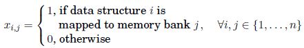
The decision variables of the problem represent the allocation of data structures to memory banks. These variables are modeled as a binary matrix X, where:
The vector of real non-negative variables Z represents the memory bank that is actually used.
The mixed integer program for that problem is the following:
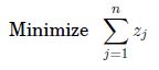
The cost function of the problem, equation [2.3], minimizes the number of memory banks used to store the data structures of the application.
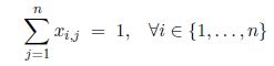
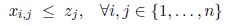
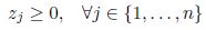
Equation [2.4] enforces that each data structure is allocated to exactly one memory bank. Equation [2.5] is used for ensuring that two data structures involved in a conflict k are assigned to different memory banks, except for the case where a data structure is conflicting with itself. Equation [2.6] sets zj to 1 if memory bank j is Equation [2.6] sets zj to 1 if memory bank j is actually used. Finally, xi,j is set as a binary variable, for all (i, j) and zj is non-negative for all j (explicit integrability enforcement is not required).
An optimal solution to the unconstrained memory allocation problem can be computed by using a solver such as GLPK [GNU 09] or Xpress-MP [FIC 09]. However, an optimal solution cannot be obtained in a reasonable amount of time (more than one h) for medium-size instances. Indeed, the following section describes that this problem is equivalent to finding the chromatic number of a conflict graph. As the chromatic number is NP-hard, so is the unconstrained memory allocation problem.
The access schedule of a particular application can be represented as a conflict graph. Figure 2.2 illustrates the conflict graph of a piece of code.
The conflict graph G = (X, U) for the unconstrained memory allocation problem is defined as follows: each vertex x in X models a data structure (array of scalars) and an edge u ∈ U models a conflict between two data structures. There are no multiple edges, that is two different conflicts between two data structures. Each auto-conflict is represented by a loop. We have an isolated vertex auto-conflict for each data structure that is not in conflict with any other data structure.
We can formulate the unconstrained memory allocation problem using this conflict graph as follows: finding the minimum number of memory banks such that two adjacent vertices are not allocated to the same memory bank.
In order to state the vertex coloring problem for our conflict graph, loops (auto-conflicts) and isolated vertices are removed. In this way, we have an undirected and simple graph. The vertex coloring problem is to assign a color to every vertex in such a way that two adjacent vertices do not have the same color, while minimizing the total number of colors used.
The chromatic number of the conflict graph is the smallest number of colors needed to color it. Consequently, memory banks can be modeled as colors, and addressing the unconstrained memory allocation problem is equivalent to finding the chromatic number of the conflict graph.
In the electronic chip CAD, the unconstrained memory allocation problem is solved repeatedly. Therefore, it is important to quickly estimate the number of memory banks required by the application. For these reasons, we are interested in upper bounds on the chromatic number. Upper bounds are of particular interest for memory management and register allocation, because they enable us to reduce the search space for non-conflicting memory/register allocations.
In the following section, we introduce the main bounds on the chromatic number found in the literature.
We give some formal definitions about the vertex coloring problem and the chromatic number. Also, we introduce some notations.
Formally, a coloring of graph G = (X, U) is a function  , where each vertex in X is allocated an integer value that is called a color. A proper coloring satisfies F (u) ≠ F(v) for all (u, v) ∈ U [DIE 05, KLO 02]. A graph is said to be α-colorable if there exists a coloring that uses, at most, α different colors. In that case, all the vertices colored with the same color are said to be part of the same class.
The smallest number of colors involved in any proper coloring G is called the chromatic number, which is denoted by χ(G). The problem of finding χ(G), as well as a minimum coloring, is NP-hard and is still the focus of an intense research effort [BUI 08, CAR 08, MEH 96, MÉN 08].
We recall some elementary results on the vertex coloring problem and chromatic number. A graph cannot be α-colorable if α < χ(G). The chromatic number equals 1, if and only if G is a totally disconnected graph, it is equal to |X| if G is complete, and for the graphs that are exactly bipartite (including trees and forests) the chromatic number is 2.
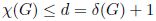
Regarding lower bounds, the chromatic number is greater than or equal to the clique number denoted by ω(G), which is the size of the largest clique in the graph, thus ω(G) ≤ χ(G). However, this bound is difficult to use in practice as finding the clique number is NP-hard, and the Lovasz number is known to be a better lower bound for χ(G) as it is “sandwiched” between the clique number and the chromatic number [KNU 94]. Moreover, the Lovasz number can be calculated in polynomial time.
Let G be a non-directed, simple graph, where n = |X| is the number of vertices and m = | U | is the number of edges. The degree of vertex i is denoted by di for all i ∈ {1, …, n}, and δ(G) is the highest degree in G. The following upper bounds on χ(G) can be found in the literature (e.g. in [LAC 03], there is a good summary about upper bounds):
 [DIE 05, GRA 11].
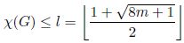 [DIE 05, GRA 11].
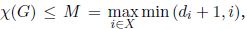 provided that d1 ≥ d2 ≥ … ≥ dn [WEL 67].
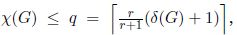 where r is the maximum number of vertices of the same degree, each at least (δ(G) + 2)/2 [STA 02].
There exists some upper bounds on the chromatic number for special classes of graphs:
In section 2.5, three new upper bounds on the chromatic number are proposed. In sections 2.6 and 2.7, the quality of these new bounds is compared with the upper bounds mentioned in this section.
For the sake of illustration of the unconstrained memory allocation problem, we present an instance based on the LMS (least mean square) dual-channel filter [BES 04], which is a well-known signal processing algorithm. This algorithm is written in C and is to be implemented on a TI-C6201 target.
Figure 2.1 shows the source code and access schedule of this LMS dual-channel filter. This schedule was generated by the compilation and code profiling tools of SoftExplorer [LAB 06], which is a software of the Lab-STICC laboratory [LAB 11].
The data structures are the arrays defined at line 10 of the C code and the constants (lines 4–8) and integer variables (line 12) are not considered for the memory allocation.
The access schedule presents the data structures in conflict. In the schedule, LD means load/read a data structure and ST means store/write in a data structure. In the sixth ordering, the processor must at the same time load data structure X1 and store in H11 the result of operation executed in line 22 of code source.
SoftExplorer separately compiles the code presented at each loop or condition instruction. The first four orderings correspond to the operations executed in for loops of the main for loop (lines 16, 19, 25 and 28).
In this example, most of the conflicts are presented in the data structures involved in the same operations. Only the fifth and eighth conflicts involve data structures used in different operations.
Moreover, the last two orderings are the auto-conflicts, it is due to the optimization rules presented in the compiler gcc used by SoftExplorer. In the main for loop, data structures X1 and X2 are present two times (see lines 22, 23, 31 and 32), so they are considered only the first time when they appear in the loop. Thus, X1 and X2 are ignored in lines 31 and 32, respectively, and data structures H21 and H22 are in conflict with themselves.
Figure 2.2 shows the conflict graph from the access schedule. Each data structure is represented by a vertex and each conflict in the schedule is represented by an edge. The auto-conflicts (loops in the graph) are represented with a dotted line, because they will be removed to state the vertex graph coloring problem. In this example, there are no isolated vertices.
Figure 2.1. Code and access schedule of LMS dual-channel filter
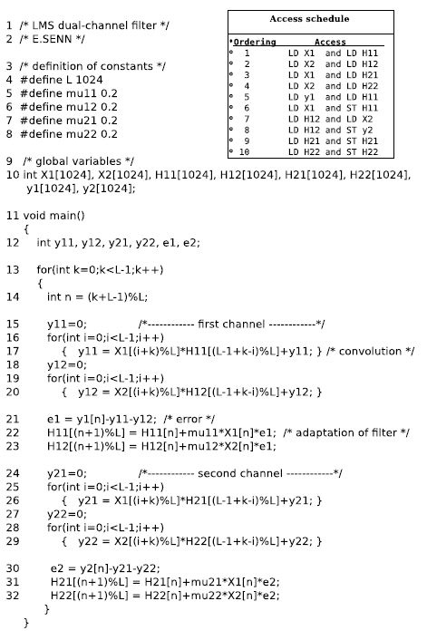
Figure 2.2. (a) Access schedule and (b) conflict graph of LMS dual-channel filter
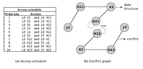
The chromatic number for the conflict graph without loops is two. Thus, it is necessary for two memory banks to find a memory allocation where all non-auto-conflicts are closed constraints.
The following lemma is required for proving Theorem 2.1, which introduces the first bound proposed.
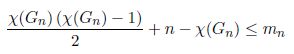
LEMMA 2.1.– The following inequality holds for any connected, simple graph Gn = (V, E), where mn = |E|.
This inequality is referred to as equation [2.9].
PROOF.– Lemma 2.1 is proved by the recurrence on n.
First, it can be observed that Lemma 2.1 is obviously true for n = 2. Indeed, there exists a unique connected, simple graph on two vertices, it has a single edge, and χ(G2) = 2.
Second, we assume that Lemma 2.1 is valid for all graphs having at most n vertices. We now prove that the inequality of Lemma 2.1 holds for any connected, simple graph on n + 1 vertices. Let such a graph be denoted by Gn+1. It has mn+1 edges and its chromatic number is χ(Gn+1).
Gn+1 can be seen as a connected, simple graph Gn plus an additional vertex denoted by n + 1, and additional edges incident to this new vertex. The addition of vertex n + 1 to Gn leads either to χ(Gn+1) = χ(Gn) or to χ(Gn+1) = χ(Gn) + 1. Indeed, the introduction of a new vertex (along with its incident edges) to a graph leads to increase in the chromatic number by at most one.
Adding 1 to equation [2.9] yields
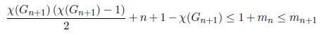
We have 1 + mn ≤ mn+1 because at least one new edge is to be added to Gn for building Gn+1: vertex n + 1 has to be connected to at least one edge in Gn for Gn+1 to be connected.
A minimum coloring of Gn+1 can be obtained by keeping the minimum coloring of Gn, and by assigning color χ(Gn+1) = χ(Gn) + 1 to vertex n + 1. Since this coloring is minimum, there exists at least one edge between any pair of color classes [DIE 05]. In particular, this requirement for color χ(Gn+1) implies that the degree of vertex n + 1 is at least χ(Gn), hence mn + χ(Gn) ≤ mn+1.
Adding χ(Gn) to equation [2.9] yields
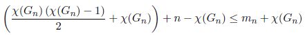
The quantity in parenthesis is equal to the sum of the integers in {1, …, χ(Gn)}, and since χ(Gn+1) = χ(Gn) + 1,
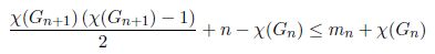
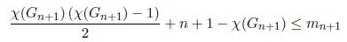
Finally, as n – χ(Gn) = n + 1 – χ(Gn+1) and mn + χ(Gn) ≤ mn+1,
THEOREM 2.1.– The following inequality holds for any connected, simple undirected graph G.
χ(G) ≤ ξ,
with 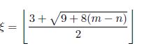
PROOF.– By Lemma 2.1, m can be lower bounded as follows:
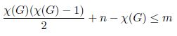
This inequality leads to the following second-order polynomial in the variable χ(G):
χ(G)2 – 3χ(G) – 2(m – n) ≤ 0
Once solved, this inequality leads to:
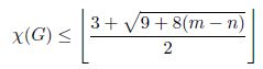
Note that because all connected graphs have at least n – 1 edges, then 8(m – n) + 9 ≥ 1, thus the square root is in R+.
REMARK 2.1.– As this bound is only based on the number of the vertices and edges in the graph, it yields the same value for all graphs having the same number of vertices and edges. This bound computation requires O(1) operations.
THEOREM 2.2.– For any simple, undirected graph G, χ(G) ≤ ζ where ζ is the greatest number of vertices with a degree greater than or equal to ζ – 1.
THEOREM 2.3.– For any simple, undirected graph G, χ(G) ≤ η, where η is the greatest number of vertices with a degree greater than or equal to η that are adjacent to at least η – 1 vertices, each of them with a degree larger than or equal to η – 1.
Before proving Theorems 2.2 and 2.3, some notations and definitions need to be stated. It should be noticed that connectivity is not required for the last two bounds, which involves more information on the graph topology than the first one.
The degree of saturation [BRÉ 79, KLO 02] of a vertex υ ∈ X denoted by DS(υ) is the number of different colors of the vertices adjacent to υ. For a minimum coloring of graph G, DS(υ) is in {1,…, χ(G) – 1} for all υ ∈ X.
The following notations are used throughout this chapter:
The last two bounds are based on the degree of saturation of a vertex and on Lemma 2.2.
LEMMA 2.2.– Let F be a minimal coloring of G. For every color k in C, there exists at least one vertex υ colored with k (i.e. F(υ) = k), such that its degree of saturation is χ(G) – 1 and where υ is adjacent to at least χ(G) – 1 vertices with a degree larger than or equal to χ(G) – 1.
PROOF OF LEMMA 2.2.– We prove the lemma by contradiction. First, we show that for all k in C, there exists a vertex υ, colored with k, such that DS(υ) = χ(G) – 1. To do so, we assume that there exists a color k in C such that any vertex υ colored with k has a degree of saturation that is strictly less than χ(G) – 1.
Then, it can be deduced that for all υ ∈ X such that F (υ) = k, there exists a color c ∈ C\{k} such that there does not exist u ∈ N(υ)/F(u) = c. Consequently, a new valid coloring can be derived from the current one by setting F(υ) = c. Indeed, υ is not connected to any vertex colored with c. This operation can be performed for any vertex colored with k, leading to a valid coloring in which color k is never used. Hence, this new coloring involves χ(G) – 1 colors, which is impossible by definition of the chromatic number.
Second, we show that, for every k in C, there exists a vertex v colored with k, whose degree of saturation is equal to χ(G) – 1, and such that υ has at least χ(G) – 1 neighbors with degree larger than or equal to χ(G) – 1. To do so, we assume that there exists a color k in C such that any vertex υ colored with k having a degree of saturation equal to χ(G) – 1 has strictly less than χ(G) – 1 neighbors with a degree larger than or equal to χ(G) – 1.
Then, it can be deduced that for every vertex υ colored with k and such that DS(υ) = χ(G) – 1, there exists one color c ∈ C/{k} such that the degree of any vertex w ∈ V(υ)/F(w) = c is strictly less than χ(G) – 1. Then, for each vertex w ∈ V(υ) / F(w) = c, there exists a color l ∈ C\{k,c} such that setting F(w) to l yields a valid coloring. As a result, color c is no longer used in N(υ), thus DS(υ) is no longer χ(G) – 1. This operation can be performed for any vertex υ such that F(υ) = k/DS(υ) = χ(G) – 1, leading to a coloring in which there is no vertex υ colored with k and such that DS(υ) = χ(G) – 1. It can then be deduced from the first part of this proof that in such a situation, G can be colored with strictly less than χ(G) colors, which is impossible.
PROOF OF THEOREM 2.2.– It can be deduced from Lemma 2.2 that there exists at least χ(G) vertices in G, with a degree at least χ(G) – 1. Thus, ζ being the greatest number of vertices with a degree greater than or equal to ζ – 1, the following inequality holds: χ(G) ≤ ζ.
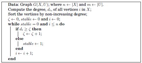
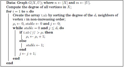
REMARK 2.2.– It can easily be seen that Algorithm 1 which returns ζ, has a computational complexity of O (max{m, n log2(n)}), as it requires enumerating the m edges to compute the degree of the vertices, n log2(n) operations to sort the vertices and ζ ≤ n iterations in the while loop.
Algorithm 1. Computing ζ
PROOF OF THEOREM 2.3.– It can be deduced from Lemma 2.1 that there exist at least χ(G) vertices in G, which are adjacent to χ(G) – 1 vertices with degrees larger than χ(G) – 1. Since n is the greatest number of vertices with a degree greater than or equal to η that are adjacent to at least η – 1 vertices, each of them with degree larger than or equal to η − 1, then χ(G) ≤ η.
REMARK 2.3.– The proposed algorithm for computing η relies on the neighboring density. The neighboring density of vertex i is denoted by ρi and is defined as follows: ρi is the largest integer such that vertex i is adjacent to at least ρi vertices. Each of the latter has a degree greater than or equal to ρi. Algorithm 2 computes the neighboring density of all vertices. Then, η is computed by executing Algorithm 1, where di is replaced with ρi for all i ∈ X and where ζ is replaced with η. The computational complexity for determining the neighboring density of all vertices is O (m log2(m)), as it requires m operations to compute the degree and 2m log2(2m) operations to sort 2m numbers (the sum of degree of all vertices is 2m). Therefore, the computational complexity for computing η is O (max{m log2(m), n log2(n)}).
Algorithm 2. Computing the neighboring density of all vertices
The three bounds introduced in this chapter are compared theoretically to the five upper bounds from the literature, which were mentioned in the introduction, namely d, l, M, s and q.
PROPOSITION 2.1.– For any simple, undirected, connected graph
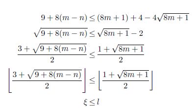
ξ ≤ l
PROOF.– The number of edges in any simple undirected graph is less than or equal to n(n – 1)/2, thus:
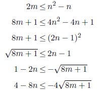
Then, 8m + 5 is added to the last inequality
PROPOSITION 2.2.– For any simple undirected graph
η ≤ ζ
PROOF.– This is obvious as the definition of ζ and η can be seen as the statement of two maximization problems. Since the requirements (or constraints) on η are more stringent than the requirements on ζ, the inequality η ≤ ζ holds.
PROPOSITION 2.3.– For any simple undirected graph
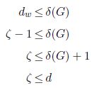
η ≤ d
PROOF.– Since δ(G) is the maximum degree in the graph, dυ ≤ δ(G) for all υ ∈ X. By definition of ζ, there exists at least one vertex w with a degree greater than or equal to ζ – 1, then:
PROPOSITION 2.4.– For any simple undirected graph
ζ = M
PROOF.– First, it is recalled that by definition of ζ, there do not exist ζ + 1 vertices with a degree larger than or equal to ζ (otherwise this would be conflicting with the definition of ζ).
It is assumed without loss of generality that the vertices are indexed by non-increasing degree: d1 ≥ d2 ≥ … ≥ dn. Then, it can be deduced that the vertices whose index is in {ζ+1,…, n} have a degree less than or equal to ζ – 1.
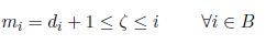
The vertex set X = {1,…, n} is split into two subsets: X = A ∪ B with A = {1,…, ζ} and B = {ζ + 1,…, n}. In other words, A is the set of the ζ vertices of highest degree and B is the set of the n – ζ vertices of lower degree.
For all i in X, we denote by mi the minimum between di + 1 and i (i.e. this makes it possible to write  ).
).
For all i ∈ X, i is either in A or in B:
If i ∈ A, then vertex i is such that di ≥ ζ – 1, that is di + 1 ≥ ζ. Moreover, by definition of A, i ≤ ζ. Consequently,
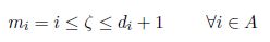
In particular, for i = ζ, mi = ζ, and by definition of M, ζ ≤ M.
Finally, the inequality mi ≤ ζ holds for all i ∈ {1,…, n} and by definition of M this leads to M ≤ ζ.
REMARK 2.4.– Computing M by using the formula M =  provided in [WEL 67] has a computational complexity of O (max{m, n log2 n}), as it requires computing the degree of the vertices and sorting them by non-increasing degree. Although ζ and M are defined differently, their computation requires the same order of arithmetical operations.
PROPOSITION 2.5.– For any simple undirected graph
η ≤ 8
PROOF.– By definition of δ2(G), there do not exist two adjacent vertices i and j in X such that di > δ2(G) and dj > δ2(G). Consequently, it is impossible to find a vertex adjacent to at least δ2(G) + 1 vertices whose degrees are at least δ2(G) + 1. This shows that η – 1 is less than or equal to δ2(G), that is η ≤ s.
PROPOSITION 2.6.– For any simple undirected graph
ζ ≤ q
PROOF.– We prove by contradiction that ζ ≤ q by using Proposition 2.4.
We denote by A and B the two subsets of X: A = {1,…,ζ} and B = {ζ + 1,…,n}.
As shown in the proof of Proposition 2.4:
We assume that ζ > q.
First, it is recalled that Stacho has proved in [STA 02] that dq < q, that is dq + 1 ≤ q. Then, ζ > q does not hold if q ∈ A.
Second, if q belongs to B, it must satisfy ζ ≤ q that is conflicting with the hypothesis ζ > q.
Consequently, this proves that ζ ≤ q.
The new bounds introduced in this chapter are compared to the five bounds of the literature on the DIMACS instances [DIM 11] for vertex coloring. The detailed results are shown in Table 2.1 for 136 instances. The first three columns of this table provide the instance source at DIMACS, its name, the number of vertices and the number of edges. The next eight columns show the upper bound on the number of colors provided by the five bounds of the literature and the three upper bounds introduced in this chapter. The last three rows of Table 2.1 show the average value of each bound on the DIMACS instances, the penultimate row provides the average deviation to η over all the other bounds (note that these figures are not computed on the average numbers of colors), and the last row is the total amount of CPU time (in seconds) required for computing each bound on an Intel® Xeon® processor system at 2.67 GHz and 8 Gbytes RAM. Algorithms have been implemented in C++ and compiled with gcc 4.11 on a Linux system.
Table 2.1. Upper bounds on the chromatic number

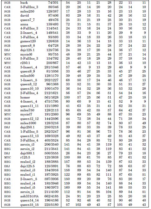
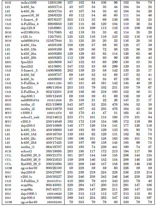
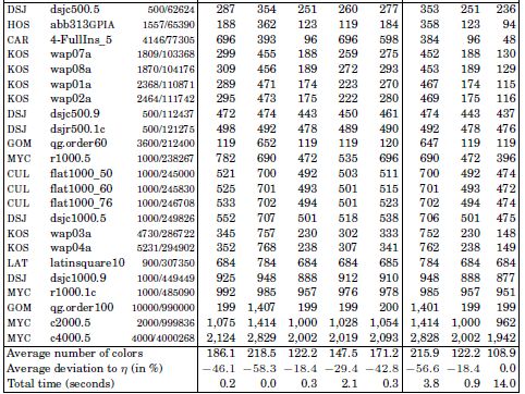
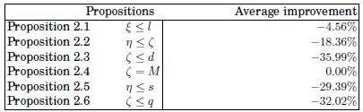
Table 2.2 is presented to assess the practical strength of Propositions 2.1–2.6. As each proposition is of the form a ≤ b (except Proposition 2.4), the last column of Table 2.2 indicates by which amount bound a is better than bound b (the average improvement is defined as the average value of (a – b)/b over all the instances, in percent). Naturally, this amount is 0% in the particular case of Proposition 2.4, as it is an equality. It can be seen that ξ does not provide a significant advantage over l in practice.
However, Propositions 2.2, 2.3, 2.5 and 2.6 are stronger as the improvement is larger than 18%. More specifically, the best bound proposed in this chapter outperforms the best upper bound of the literature by more than 18% on average. Proving that M = ζ is important for highlighting the reason for the practical superiority of η over M. Indeed, η is based on the same principle as ζ, it focuses on the degrees of saturation of vertices. The difference is that η goes one step further than ζ by considering the degree of saturation of the neighbors of each vertex (i.e. the so-called neighboring density). This additional requirement has a computational cost that is drastically larger than the one required by computing ζ, but it provides a significant improvement in terms of the upper bound quality.
Table 2.2. Computational assessment of Propositions 2.1–2.6 based on Table 2.1
In this chapter, we have presented the first version of the memory allocation problem. This problem is equivalent to finding the chromatic number of the application’s conflict graph. Three new upper bounds on the chromatic number have been introduced. The proposed upper bounds do not make any assumptions on the graph structure, they are based on basic graph characteristics such as the number of vertices, edges and vertex degrees.
The first upper bound, ξ, is based on the number of edges and vertices and only requires connectivity, whereas the last bounds, ζ and η, are based on the degree of the vertices in the graph.
We have theoretically and computationally assessed our upper bounds with the bounds of the literature. It has been shown that ζ is equal to an existing bound, while being computed in a very different way. Moreover, a series of inequalities has been proved, showing that these new bounds outperform five of the most well-known upper bounds from the literature. Computational experiments also have shown that the best bound proposed, η, is significantly better than the five bounds of the literature, and highlight the benefit of using the degree of saturation and its refined version (the neighboring density) for producing competitive upper bounds for vertex coloring. Indeed, using more information on graph topology appears to be a promising direction for future work.
The upper bounds on the chromatic number introduced in this chapter appear to be both significantly better than the literature bounds, and easily computable even for large graphs. However, there exist sophisticated metaheuristics for the vertex coloring problem (see e.g. [XIK 07, POR 10, HER 08, COJ 06, GON 02]), and advanced bounds (see e.g. [BUI 08, CAR 08, MEH 96, MÉN 08]) that reach better results than ours. But the computational time for getting these results and the associated coloring is sometimes longer than 20 minutes, which is far too long for the CAD electronic chip design in which the problem is solved. Indeed, memory allocation is only one part of the electronic chip design process, which is split in a series of sequential steps. Furthermore, as many design variations may be considered, the memory allocation problem has to be solved repeatedly, and CAD softwares are expected to be reactive enough to allow for “what if” studies. In conclusion, our bounds provide useful information for electronic designers. If the number of memory banks is greater than the minimum over ξ, ζ and η, then electronic designers are guaranteed to find a memory allocation where all non-auto-conflicts are closed.
The first two upper bounds were presented at the 2009 Cologne-Twente Workshop on Graphs and Combinatorial Optimization (see [SOT 09]), and a paper introducing the three new upper bounds by Discrete Applied Mathematics was published in 2011 [SOT 11b].