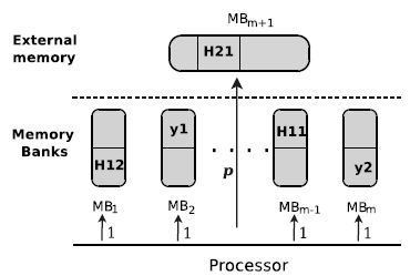
Figure 4.1. The memory architecture for MemExplorer
This chapter addresses the third version of the memory allocation problem. This problem is related to the data binding problems described in the state of the art, section 1.3.3. The general objective is the allocation of the data structures from a specific application to a given memory architecture. Compared to the problem of the previous chapter, additional constraints on the memory banks and data structures are considered. Moreover, an external memory is now present in the target architecture.
The metaheuristics designed for the previous version of the memory allocation problem are no longer used for addressing the problem of this chapter, because they require too much CPU time to return good solutions. This chapter discusses an exact approach and a variable neighborhood search (VNS)-based metaheuristic to tackle the general memory allocation problem. Numerical experiments are conducted on a set of instances, and statistical analysis is used to assess the results. The proposed metaheuristic appears to be suitable for the electronic design needs of today and tomorrow.
The general memory allocation problem, called MemExplorer, is discussed in this chapter. This problem is focused on the allocation of the data structures from a given application to a given memory architecture. MemExplorer is more realistic than the previous version of the memory allocation problem presented in Chapter 3. In addition to memory banks, an external memory is considered in the target architecture. External memories store the long-term data, and they improve the throughput of an embedded system [NAC 01].
In this problem, the number of memory banks is fixed and the memory bank capacities are limited. The sizes of data structures and the number of accesses to them are both taken into account. Moreover, the time for accessing to the external memory is also considered.
In the data binding problem presented in section 1.3.3, we have mentioned some works that consider the capacities of memory banks and the number of accesses to data structures, and other works that use an external memory bank in the target architecture. Although MemExplorer has some similarities with the data binding problems, it is not equivalent to any of them. This is mainly due to the fact that the architecture, the constraints and the objective function are all different.
Assumptions similar to those in the previous version of memory allocation are considered in this problem. It is assumed that the application to be implemented (e.g. MPEG encoding, filtering and other signal processing algorithms) is provided as a C source code, and the data structures involved have to be mapped into memory bank. And all memory banks can be accessed simultaneously.
Hence, a conflict between two data structures is defined as in Chapters 2 and 3, and the cost of conflicts is also taken into account. A conflict is open when its data structures are allocated to the same memory bank, so a cost is generated. A conflict is closed when the conflicting data structures are mapped in different memory banks, so no cost is generated.
Due to cost and technological reasons, the number and the capacity of memory banks are limited; an external memory with unlimited capacity is then assumed to be available for storing data (it models the mass memory storage).
The processor requires access to data structures in order to execute the operations (or instructions) of the application. The access time to data structure is expressed in milliseconds (ms), and depends on its current allocation. If a data structure is allocated to a memory bank, its total access time is equal to the number of times the processor accesses it, because the transfer rate from a memory bank to the processor is 1 ms. If a data structure is allocated to the external memory, its access time is equal to its number of accesses multiplied by p ms, because the transfer rate from the external memory to the processor is p ms.
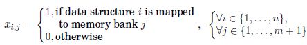
Figure 4.1 shows the memory architecture considered for this problem.
A good management of memory allocation allows decreasing the energy consumption. In fact, electronic practitioners consider that to some extent, minimizing power consumption is equivalent to minimizing the running time of an application on a given architecture [CHI 02]. As a result, memory allocation must be such that the loading operations are performed in parallel as often as possible. With this aim, the general memory allocation problem is stated as follows: for a given number of capacitated memory banks and an external memory, we search for a memory allocation for data structures such that the time spent accessing these data is minimized. Section 4.3 presents an instance of MemExplorer aimed at exemplifying this problem.
Figure 4.1. The memory architecture for MemExplorer
Electronics practitioners often left to the compiler the management of the data structures into memory banks. Nevertheless, the solution found by the compiler is often too far from the optimal memory allocation. In this work, we seek for better alternatives to manage the general memory allocation problem. Hence, an integer linear program is designed for MemExplorer in the following section. In section 4.4, we discuss metaheuristics conceived for this problem. The results produced by the exact method and heuristic approaches are presented, and statistically compared in section 4.5.
The number of memory banks is denoted by m. Memory bank m + 1 refers to the external memory. The capacity of memory bank j is cj for all j ∈ {1,…,m} (it is recalled that the external memory is not subject to capacity constraint).
The number of data structures is denoted by n. The size of a data structure i is denoted by si for all i ∈ {1,…,n}. Besides its size, each data structure i is also characterized by the number of times that the processor accesses it, it is denoted by ei for all i ∈ {1,…,n}. ei represents the time required to access data structure i if it is mapped to a memory bank. If a data structure i is mapped to the external memory its access time is equal to p × ei.
Conflict k is associated with its conflict cost dk, for all k ∈ {1,…,o}, where o is the number of conflicts.
Sizes and capacities are expressed in the same memory capacity unit, typically kilobytes (kB). Conflict costs and access time are expressed in the same time unit, typically milliseconds.
The isolated data structures, and the case where a data structure is conflicting with itself are both taken into account for the ILP formulation and for the proposed metaheuristics.
There are two sets of decision variables; the first set represents the allocation of data structures to memory banks. These variables are modeled as a binary matrix X, where:
The second set is a vector of real non-negative variables Y, which models the conflict statuses; so variable yk associated with conflict k has two possible values:
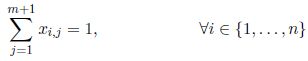
The mixed integer program for the general memory allocation problem is as follows:
The cost function of the problem, equation [4.3], is the total time spent accessing the data structures and storing them in the appropriate registers to perform the required operations listed in the C file. It is expressed in milliseconds.
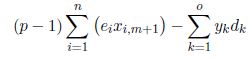
This cost function is the sum of three terms. The first term is the cost generated by accessing to data structures into memory banks, whereas the second term is the cost produced by accessing to data structures placed in the external memory. The last term is the sum of the closed conflicts. Note that all conflict costs are involved in the sum of the first two terms. The last term is negative, and thus, only the open conflicts are presented in the objective function.
Because 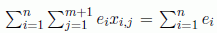 is a constant value, it is equivalent to minimize:
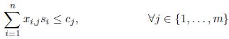
Equation [4.4] enforces that each data structure is allocated either to a unique memory bank or to the external memory. Equation [4.5] is used for ensuring that the total size of the data structures allocated to a memory bank does not exceed its capacity. For any conflict k, variable yk must be set appropriately; this is enforced by equation [4.6]. For an auto-conflict k, yk is equal to 1. Finally, xi,j is a binary variable, for all (i, j), and yk is non-negative for all k.
The number of memory banks with their capacities, the external memory and transfer rate p ms describe the architecture of the chip. The number of data structures, their size and access time describe the application, whereas the conflicts and their costs carry information about both the architecture and the application.
Note that this problem is similar to the k-weighted graph coloring problem [CAR 66] if memory banks are not subject to capacity constraints, or if their capacity is large enough for holding all the data structures. In fact, in that case the external memory is no longer used and the size, as well as the access cost of data structures, can be ignored.
An optimal solution to MemExplorer problem can be computed by using a solver such as GLPK [GNU 09] or Xpress-MP [FIC 09]. However, as shown by the computational tests in section 4.5, an optimal solution cannot be obtained in a reasonable amount of time for medium-size instances. Moreover, MemExplorer is NP-hard, because it generalizes the k-weighted graph coloring problem [CAR 66].
In the following section, we propose a VNS-based metaheuristic for addressing this problem. Vredeveld and Lenstra [VRE 03] address the k-weighted graph coloring problem by local search programming. We compare the results reached by ILP formulation, our metaheuristic approaches and local search programming in section 4.5. Moreover, we use a statistical test to analyze the performance of these approaches.
This is an instance produced from a least mean square (LMS) dual-channel filter [BES 04]. It exemplifies the general memory allocation problem. The information yield from the compilation and code profiling of this signal processing algorithm are shown in Table 4.1. To this end, we have used the software of LAB-STICC, SoftExplorer [LAB 06].
Table 4.1. Conflicts and data structures of LMS dual-channel filter
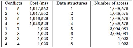
All data structures have the same size of 15,700 kB. The memory architecture has two memory banks with capacity of 47,100 kB. Memory banks can only store three data structures. On the target architecture, p is equal to 16 ms. Figure 4.2(a) shows the solution found by solving the ILP formulation using the solver Xpress-MP. Figure 4.2(b) illustrates the solution.
In the optimal solution, the data structures that are least accessed are allocated in the external memory. Thus, only auto-conflicts are open. The cost generated by this solution is formed by:
Figure 4.2. An optimal solution for the example of MemExplorer
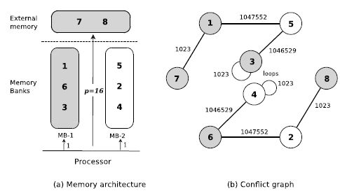
Access time to memory banks:  = 8,382,462 ms
Access time to external memory:  = 32,736 ms
Access time saved by closed conflicts:  = 4,190,208 ms
Hence, the total cost of the optimal solution is 4,224,990 ms.
In this section, we describe the design of the different metaheuristics used for addressing this problem. Before presenting the metaheuristics for MemExplorer, we present the algorithms used for generating initial solutions, as well as two neighborhoods. Then, a tabu search-based approach is described with the two neighborhoods for exploring the solution space. At the end of this section, a variable neighborhood search-based approach hybridized with a tabu search-inspired method is also presented.
Here, we present two ways for generating initial solutions. The first of these generates feasible solutions at random, and the second builds solutions using a greedy algorithm.
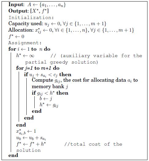
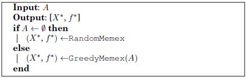
Algorithm 6 presents the procedure RandomMemex for generating random feasible initial solutions. At each iteration, a data structure is allocated to a random memory bank (or the external memory) provided that capacity constraints are satisfied.
GreedyMemex is a greedy algorithm for MemExplorer, this kind of algorithm makes locally optimal choices at each stage in the hope of finding the global optimum [BLA 05, COR 90]. Generally, greedy algorithms do not reach an optimal solution because they are trapped in local optima, but they are easy to implement and can provide initial solutions to more advanced approaches.
GreedyMemex is described in pseudo-code of Algorithm 7, where A is a permutation of the set {1,…,n} that models data structures, used for generating different solutions. Solution X* is the best allocation found by the algorithm, where  variables have the same meaning as in equation [4.1], and f* = f (X*). Matrix G is used to assess the cost when data structures are moved to different memory banks or to the external memory. More precisely, gi,j is the sum of all open conflict costs produced by assigning data structure i to memory bank j. If data structure i is moved to external memory (j = m + 1), gi,j is the sum of all open conflict costs multiplied by p plus its access time multiplied by (p − 1). The numerical value of gi,j depends on the current solution because the open conflict cost depends on the allocation of the other data structures.
Algorithm 6. Pseudo-code for RandomMemex
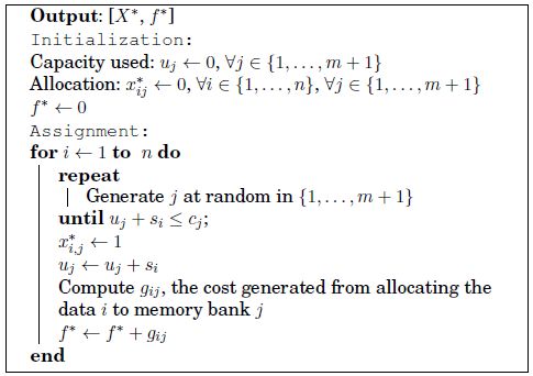
At each iteration, GreedyMemex completes a partial solution that is initially empty by allocating the next data structure in A. The allocation for the current data structure is performed by assigning it to the memory bank leading to the minimum local cost denoted by h*, provided that no memory bank capacity is exceeded. The considered data structure is allocated to the external memory if no memory bank can hold it. Allocation cost f* is returned when the all data structures have been allocated.
Algorithm 7. Pseudo-code for GreedyMemex
GreedyMemex has a computational complexity of O(nm). Both algorithms require very few computational efforts, but return solutions that may be far from the optimality. However, these procedures are not used as standalone algorithms, but as subroutines, as called in Algorithm 8 for generating initial solutions for a tabu search-based procedure.
Algorithm 8. Pseudo-code for InitialMemex
A tabu search method for MemExplorer is described in Algorithm 9, which is based on TabuCol, an algorithm for graph coloring described in [HER 87]. The main difference with a classic tabu search is that the size of the tabu list is not constant over time. This idea is discussed in [BAT 94] and also used in the work of Porumbel, Hao and Kuntz on the graph coloring problem [POR 09b]. In TabuMemex, the size of the tabu list NT is set to a + NT max × t every NT max iterations, where a is a fixed integer and t is a random number in [0, 2].
A pair (i, j) means that data structure i is in memory bank j. A move is a trio (i, h, j), this means that data structure i, which is currently in memory bank h, is to be moved to memory bank j. As a result, if the move (i, h, j) is performed, then the pair (i, h) is appended to the tabu list. Thus, the tabu list contains the pairs that have been performed in the recent past and it is updated on the first in first out (FIFO) basis.
The algorithm takes an initial solution X as input that can be returned by the procedure InitialMemex. Its behavior is controlled by some calibration parameters, such as the number of iterations, N iter, and the number of iterations for changing the size of the tabu list, NT max. The result of this algorithm is the best allocation found X* and its cost f*.
Algorithm 9. Pseudo-code for TabuMemex
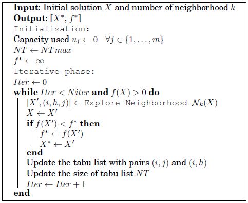
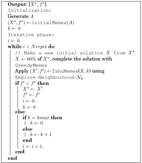
The iterative phase searches for the best solution in the neighborhood of the current solution. The neighborhood exploration is performed by calling Explore-Neighborhood-Nk(X), which calls the corresponding procedure with only one neighborhood used at a time. Two neighborhoods, denoted by N0 and N1 are considered; they are discussed in the following section. The fact that the new solution may be worse than the current solution does not matter because each new solution allows unexplored regions to be reached, and thus to escape local optima. This procedure is repeated for N iter iterations, but the search stops if a solution without any open conflict, and for which the external memory is not used, is found. In fact, such a solution is necessarily optimal because the first and third terms of equation [4.3] are zero because no conflict cost has to be paid, and no data structure is in the external memory. Consequently, the objective function assumes its absolute minimum value, the second term of equation [4.3], and so is optimal. A new solution is accepted as the best one if its total cost is less than the current best solution.
This tabu search procedure will be used as a local search procedure in a VNS-based algorithm described in section 4.4.4.
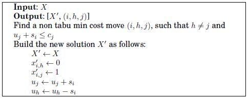
In this section, we present two algorithms that explore two different neighborhoods for MemExplorer. Both of them return the best allocation (X') found along with the corresponding move (i, h, j) performed from a given solution X. In these algorithms, a move (i, h, j) is said to be non-tabu if the pair (i, j) is not in the tabu list. Algorithm 10 explores a neighborhood that is generated by performing a feasible allocation change of a single data structure.
Algorithm 10. Pseudo-code for Explore-Neighborhood–N0
Algorithm 11 presents the Explore-Neighborhood-N1. It explores solutions that are beyond N0 by allowing the creation of infeasible solutions before repairing them.
Algorithm 11. Pseudo-code for Explore-Neighborhood-N1
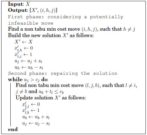
The first phase of Explore-Neighborhood-N1 performs a move that may make the current solution X' infeasible by violating the capacity constraint of a memory bank. However, this move is selected to minimize the cost of the new solution, and is not tabu. The second phase restores the solution not only by performing a series of reallocations for satisfying capacity constraints but by also trying to generate the minimum allocation cost. Then, it allows both feasible and infeasible regions to be visited successively. This way of using a neighborhood is referred to as Strategic Oscillation in [GLO 97].
Because both neighborhoods have their own utility (confirmed by preliminary tests), it seems clear that they should be used together in a certain way. The general variable neighborhood search [MLA 97] scheme is probably the most appropriate method to properly deal with several neighborhoods.
Algorithm 12 presents the VNS-based algorithm for MemExplorer. The number of neighborhoods is denoted by kmax, and the algorithm starts exploring N0 as N0 ⊂ N1.
The maximum number of iterations is denoted by N repet. Vns-Ts-MemExplorer, at each iteration, generates a solution X′ at random from X. It copies the allocation of 60% of the data structures in the initial solution (60% of the data structures are selected randomly), and the GreedyMemex is used for mapping the remaining 40% of unallocated data structures for producing a complete solution X′.
This VNS algorithm relies on two neighborhoods. N0 is the smallest neighborhood, because it is restricted to feasible solutions only. If TabuMemex improves the current solution, it keeps searching for new solutions in that neighborhood. Otherwise, it does not accept the new solution and changes the neighborhood (i.e. by applying Explore-Neighborhood-N1 to the current solution).
Algorithm 12. Pseudo-code for Vns-Ts-MemExplorer
This section presents the relevant aspects of the implementation of the algorithms. It also presents the information about the instances used to test our algorithms. Moreover, the results reached by our algorithms are presented and compared with the ILP formulation and the local search method.
There are 43 instances for testing our algorithms, they are split into two sets of instances. The first one is a collection of real instances provided by LAB-STICC laboratory [LAB 11] for electronic design purposes. These instances have been generated from their source code using the profiling tools of SoftExplorer [LAB 06]. This set of instances is called LBS.
The second set of instances originates from the Center for Discrete Mathematics and Theoretical Computer Science (DIMACS) [POR 09a], a well-known collection of online graph coloring instances. The instances in Digital Mapping Camera (DMC) have been enriched by generating edge costs at random so as to create conflict costs, access times and sizes for data structures, and also by generating a random number of memory banks with random capacities. This second set of instances is called DMC.
Although real-life instances available today are relatively small, they will become larger and larger in the future as market pressure and technology tend to integrate more and more complex functionalities in embedded systems. Moreover, industrialists do not want to provide data about their embedded applications. Thus, we tested our approaches on current instances and on larger (but artificial) ones as well, for assessing their practical use for forthcoming needs.
Algorithms have been implemented in C++ and compiled with gcc 4.11 on an Intel® Pentium IV processor system at 3 GHz and 1 gigabyte RAM.
In our experiments, the size of the tabu list is set every NT max = 50 iterations to NT = 5 + NT max × t, where t is a real number selected at random in the interval [0, 2]. The maximum number of iterations has been set to N iter = 50,000.
For the initial solutions, we have used three different sorting procedures for permutation A of data structures. Then, we have three GreedyMemex algorithms: in the first algorithm, A is not sorted. In the second algorithm, A is sorted by decreasing order of the maximum conflict cost involving each data structure and in the third, A is sorted by decreasing order of the sum of the conflict cost involving each data structure. Hence, we have four initial solutions (random initial solutions and greedy solutions) and three ways of mapping the 40% of solution X′ in VNS algorithm.
However, other tests showed that the benefit of using different initial solutions and different greedy algorithms to generate X′ is not significant. In fact, this benefit is visible only for the most difficult instances with a low value of 1.2% on average, and for the other instances, VNS algorithm finds the same solutions, no matter the initial solution or greedy algorithm.
The k-weighted graph coloring problem can be addressed by local search programming [VRE 03]. Thus, we have tested the local search on instances of MemExplorer, with the aim of comparing our algorithms with another heuristic approach. The result produced by the solver LocalSolver 1.0 [INN 10] is also reported.
The ILP formulation solved by Xpress-MP is used as a heuristic when the time limit of one hour is reached: the best solution found so far is then returned by the solver. A lower bound found by the solver was also calculated, but it was far too low for being useful.
The cost returned by Vns-Ts-MemExplorer is the best results obtained over all the combinations of different initial solutions and different greedy algorithms for generating a solution X′.
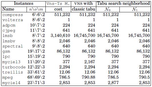
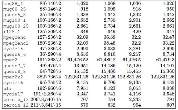
For a clear view of the difficulty, the instances have been sorted in non-decreasing order of number of conflicts. In Table 4.2, the first three columns show the main features of the instances (the source, the name, n: the number of data structures, o: the number of conflicts and m: the number of memory banks). The next two columns report the cost (in milliseconds) and CPU time (in seconds) of Vns-Ts-MemExplorer, the two following columns show the cost and CPU time of local solver and the last three columns display the results of the ILP model: lower bound, cost and CPU time.
Vns-Ts-MemExplorer results are compared with local solver programming and the ILP formulation is solved by Xpress-MP. Bold figures in Table 4.2 represent the best-known solutions over all methods. In the ILP columns, the cost with an asterisk has been proved optimal by Xpress-MP. Vns-Ts-MemExplorer reaches the optimal solution for all of the instances for which the optimal cost is known. The optimal solution is known for 88% of the real electronic instances and for 31% of the DIMACS instances. Furthermore, Vns-Ts-MemExplorer always finds a better allocation cost than Xpress-MP. The number of best solutions reported by our approach is 38, compared to 16 with a local solver and 24 with the ILP model.
Table 4.2. Vns-Ts-MemExplorer, local solver and ILP results
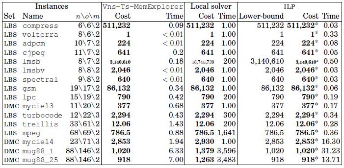
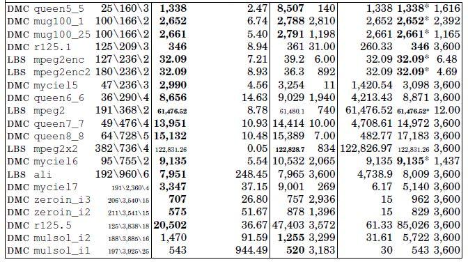
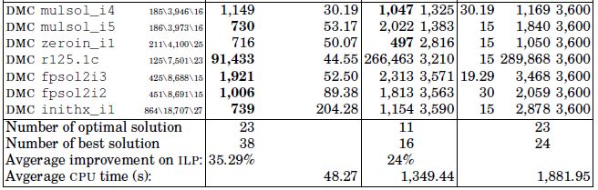
In fact, on average, the ILP cost is improved by 35.29% using the VNS algorithm, whereas a local search can either improve the cost by 24% or gets worse by the cost of 71%. CPU time comparison of Vns-Ts-MemExplorer and ILP shows that our algorithm remains significantly faster than ILP in most cases. On average, the time spent by Xpress-MP is 1,700 times longer than the time spent by VNS algorithm. When no optimal solution is found with Xpress-MP, the lower bound on the objective value seems to be of poor quality, because it is 37% more than the best solution found on average. This suggests that after one hour of computation, the optimal solution would still require a very long time to be found or to be proven. For the instances for which the optimal solution is not known, the lower bound is often far from the best known solution. It is also important to note that the ILP performs well on small-size instances (up to 250 conflicts) because it benefits from very performant advances in its code (such as internal branch-and-cut, cut pool generation and presolver).
In the VNS, the search is intensified by using TabuMemex as a local search procedure in the solution space. To assess the benefit of this strategy, we have tested our VNS with a classic tabu search method (i.e. without changing the size of the tabu list), and we have also tested TabuMemex with each neighborhood.
Table 4.3 shows the comparison between Vns-Ts-MemExplorer performances, a VNS variant with the classical tabu search and the tabu search alone with each of the two neighborhoods. The first two columns of Table 4.3 are the same as in Table 4.2, the next four columns report the cost value of each variant of the approach.
Table 4.3. Intensity of some local search variants
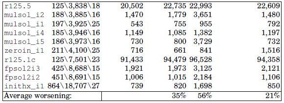
The costs reached by the other variants of VNS are worse in most cases, in fact, the solution cost of Vns-Ts-MemExplorer with classic tabu search is on average 35% higher than with TabuMemex; in addition, the tabu searches with each neighborhood (namely N0 and N1) are on average 56% and 21% worse than Vns-Ts-MemExplorer, respectively. This shows the benefit of the joint use of different neighborhoods and an advanced tabu search method.
In this section, we use a statistical test to identify differences in the performance of heuristics. In addition, we perform a post hoc paired analysis for comparing the performance between two heuristic approaches. This allows for identifying the best approach.
We have used the Friedman test [FRI 37] to detect differences in the performance of three heuristics (Vns-Ts-MemExplorer, local search, ILP formulation) using the results presented in Table 4.2.
As the results over instances are mutually independent and costs as well as CPU times can be ranked, we have applied the Friedman test for costs and CPU times. This allows us to compare separately (univariate model [CHI 07]) the performance in terms of solution quality and running time.
For each instance, the CPU times of the three approaches are ranked as follows. The smallest CPU time is ranked 1, the largest is ranked 3. If two CPU times are equal, their rank is computed as the average of the two candidate ranks (i.e. if two CPU times should be ranked 1 and 2, the rank is 1.5 for both). The same is performed for solution objective value.
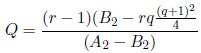
The number of instances is denoted by r, the number of compared metaheuristic is denoted by q and the Friedman test statistic is denoted by Q, it is defined as follows:
where A2 is the total sum of squared ranks and B2 is the sum of squared Ri divided by q. Ri is the sum of ranks of metaheuristics i for all i in {1,…,q}.
The null hypothesis supposes that for each instance the ranking of the metaheuristics is equally likely. The null hypothesis is rejected at the level of significance α if Q is greater than the 1 − α quantile of the F(q1,q2)-distribution (Fisher–Snedecor distribution) with q1 = q − 1 and q2 = (q − 1)(r − 1) degrees of freedom.
The test statistic Q is 21.86 for the running time, and 13.52 for the cost. Moreover, the value for the F(2,84)-distribution with a significance level α = 0.01 is 4.90. Then, we reject the null hypothesis for running time and cost at the level of significance α = 0.01.
We can conclude that there exists at least one metaheuristic whose performance is different from at least one of the other metaheuristics. To know which metaheuristics are really different, it is necessary to perform an appropriate post hoc paired comparisons test.
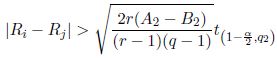
As the null hypothesis of the Friedman test was rejected, we can use the following method for knowing if two metaheuristics are different [CON 99]. We say that two metaheuristics are different if:
where  is the
  quantile of the t-distribution with (r − 1)(q − 1) degrees of freedom.
For α = 0.01, t(0.095,84)-distribution is 2.64; then, the left-hand side of equation [4.11] for the running time is 20.06 and for the cost is 17.44. Table 4.4 summarizes the paired comparisons for the cost and the running time. The bold values in the table show that the metaheuristics are different.
Table 4.4. Paired comparisons for MemExplorer
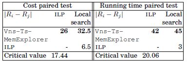
The post hoc test shows that ILP and local search have the same performance in terms of solution cost and CPU time, whereas Vns-Ts-MemExplorer is the best approach in terms of solution cost and computational time.
In this chapter, an exact approach and a VNS-based metaheuristic are proposed for addressing a memory allocation problem. Vns-Ts-MemExplorer takes advantage of some features of tabu search methods initially developed for graph coloring, which is efficient as relaxing capacity constraints on memory banks leads to the k-weighted graph coloring problem. Vns-Ts-MemExplorer appears to be performing well because of its reasonable CPU time for large instances, and because it returns an optimal memory allocation for all instances for which the optimal cost is known. These results allow one to hypothesize that the solutions found for the instances for which the optimal solution is unknown are of good quality. The improvements over a classic tabu search approach, such as the implementation of a variable tabu list, have a significant impact on solution quality. These features have TabuMemex exploring the search space efficiently.
Vns-Ts-MemExplorer achieves encouraging results for addressing the MemExplorer problem due to its well-balanced (intensification/diversification) search. The search is diversified by exploring the largest neighborhood when a local optimum is found, in addition, the local search method (TabuMemex) gives a more intensive search because of the significant improvements over a classic tabu search procedure. Using methods inspired by graph coloring problems can be successfully extended to more complex allocation problems for embedded systems, thereby accessing the gains made by using these methods to specific cases in terms of energy consumption. Moreover, it gives promising perspectives for using metaheuristics in the field of electronic design.
Finally, if the exact approach is suitable for today’s applications, it is clearly not for tomorrow’s needs. In fact, the best solution returned by the solver is generally very poor even after a long running time, and the quality of the lower bound is too bad to be at all helpful. The proposed metaheuristics appear to be suitable for the needs of today and tomorrow. The very modest CPU time compared to the exact method is an additional asset for integrating them to CAD tools, letting designers test different options in a reasonable amount of time.
The work presented in this chapter has been published in the Journal of Heuristics [SOT 11a] in 2011.