This section first introduces the target architecture used (i.e. the processor and the memory hierarchy) and then presents the estimation flow (parameters extraction), in particular, the determination of the memory conflict graph (MCG) that allows us to compute the cost of each memory access by using the cost library.
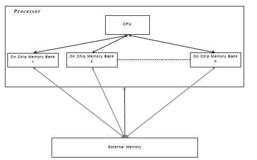
Figure 6.1 presents the generic architecture used in the modeling scheme. This architecture is composed of one processor, n on-chip memory banks (with n ≥ 0) that can be accessed by the processor to load/store its data and one external memory that can also store data (typically, the data that cannot be stored into the on-chip memory).
This type of memory architecture is often used in embedded systems because the scratchpad memories have the advantage of consuming less power than cache memories. On the one hand, the n on-chip memory banks are fast but small-sized memories, mostly a few hundred kilobytes. On the other hand, the external memory is far larger but significantly slower. Indeed, the typical access time of this kind of memory is some milliseconds, whereas on-chip memory access time is of a few nanoseconds. These features play a key role in memory mapping: if the size of a data structure exceeds the on-chip memory bank capacity, then it has to be allocated to the external memory. Furthermore, even a data structure whose size is less than the on-chip memory bank capacity may be allocated to the external memory bank if the available on-chip memory bank capacity is not large enough.
Besides memory capacity, memory access time is also an important parameter: a data structure that is often accessed by the application should be placed in the on-chip memory bank otherwise the whole application execution could be delayed.
These features (memory capacity and access time) are stored in a memory library for each memory type. This library enables MemExplorer users to get the best memory mapping to fit their architecture.
The first step in the MemExplorer design flow is to extract two types of information from the application. The first type is the size (in byte) of all data structures used in the application and the second type is the cost of all conflicts involving the data structures. These extractions are performed automatically from the application source code, this is achieved by a modified version of a GNU Compiler Collection (GCC) compiler front end.
The MemExplorer design flow is shown in Figure 6.2.
Figure 6.1. Generic architecture
Figure 6.2. MemExplorer design flow
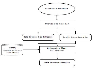
The entry point of the MemExplorer flow is a C source code provided by the user. This code is parsed by the modified front end of GCC 4.2. This parsing yields the size of each data structure (pointers are also taken into account) and the conflict graph that points out which structures are accessed in parallel. These parallel accesses generate access conflicts if the structures are mapped into the same on-chip memory bank or are both mapped into the external memory, or if one data structure is allocated an on-chip memory bank and the other data structure is allocated the external memory.
For each type of memory hierarchy, the library contains the delay costs generated by the access conflicts. Of course, these costs depend on the memory type used (on-chip or off-chip, shadow random access memory (SRAM), synchronous dynamic random access memory (SCRAM) and so on); they also depend on the processor used since the memory (on-chip or off-chip) access time differs from one processor to another. When the conflict graph and the data structure size extraction are completed, the mathematical model uses this information and the cost metric library (as presented in Figure 6.2) in order to generate the optimal data structure mapping.
This section introduces some small examples to illustrate the MCG extraction and its associated semantic.
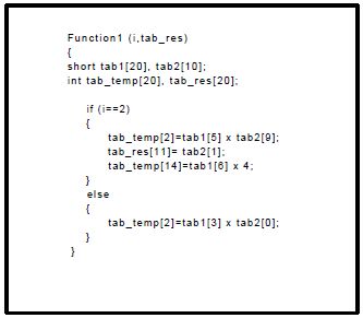
Figure 6.3 shows a brief application where only four data structures are used. These structures (which are arrays) are accessed in reading and/or writing mode.
Figure 6.3. Code Example 1
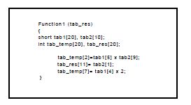
The first step taken by the front end (developed from GCC 4.2) is to extract the size of each data structure used in the application. This extraction is performed from the C code provided by the user. In the example provided (see Figure 6.3), we have to extract the size of the four data structures: tab1, tab2, tab_res, tab_temp. The first two data structures in this application are structures of short type, where a short is assumed to be a 2-byte word. Thus, tab1 has 20 elements of 2 bytes so its size is 40 bytes (the size of tab2 is 20 bytes). tab_res and tab_temp have a size of 80 bytes, so all the elements of these structures are represented using 4 bytes; an int element being coded in 32 bits in this example (the int size depends on the data bus size of the processor used).
The second step consists of analyzing all the possible access conflicts (in writing and/or reading mode) between the different data structures: these conflicts appear in the MCG. Figure 6.4 shows the MCG for the first example. It can be seen that tab1 and tab2 are conflicting and that this conflict has a cost of one. The cost of this conflict corresponds to the memory accesses performed in the first instruction of the provided example and we suppose that the load accesses are realized first. The cost carried by the arcs represents the maximum number of access conflicts. Similarly, we can determine the cost of each arc of the MCG. Finally, we can determine that tab1 and tab_res are conflicting with an associated cost of one and that tab2 and tab_temp are also in conflict with the same cost.
This first example shows a very simple case where no loops and/or control structures (if, else, switch and so forth) are used. If such control or loop structure is used in the application, we undertake the following. Each liner instruction block (LIB) is considered separately and defines the memory conflicts by taking into account the iteration numbers (for the loops) and the probability to take each branch of control structures (for the if, else…). The second example (see Figure 6.5) shows a part of this rule application when there are control structures in the C code.
Figure 6.4. Memory conflict graph: Example 1
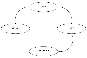
Figure 6.5. Code Example 2
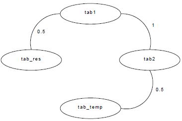
In Figure 6.6, we can see that there are three possible conflicts: the first one between tab1 and tab_res with a cost of 0.5, the second between tab2 and tab_temp with the same cost and the last one between tab1 and tab2 with a cost of one. This last conflict is twice more costly than the others because a conflict exists between these two data not only in the if branch but also in the else one. So, as the probability to take each branch of the control structure is the same in this example (by default, the two branches have the same probability), each conflict (in the if and the else branches) can occur one time with a probability of 0.5. In conclusion, each conflict has a cost of 0.5, so the addition of these costs is carried by one arc whose cost is one. The MemExplorer user can change the execution probabilities of each control branch by using pragma inserted into the C code. These pragma are used by our tool but are not taken into account during the compilation step (as with code comments).
Figure 6.6. Memory conflict graph: Example 2
Finally, the third example (see Figure 6.7) shows an application using loops and control structures.
In Figure 6.8, there are three memory conflicts: the first one between tab1 and tab2 with a cost of 7.5, the second between tab2 and tab_temp with the same cost and the third conflict between tab1 and tab_res with a cost of 12.5. Each cost is computed by using both the iteration number of loops, in which the conflicts are generated, and the probability to execute the branch control. In this example, the probability to execute the if branch is equal to 0.75 (normalized to one) because the user annotated the C code thus the probability to execute the else branch is then equal to 0.25 (MemExplorer computes the else probability by subtracting 0.75 from one so, the user does not need to annotate the else). Furthermore, the iteration number of the first loop is equal to 10 so the first conflict between tab1 and tab2 is computed as follows:
Conflict Cost = 0.75 × 10 = 7.5
Figure 6.7. Code Example 3
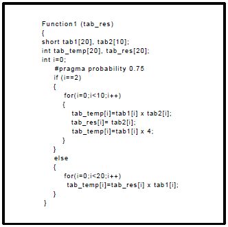
Figure 6.8. Memory conflict graph: Example 3
A node in the graph (which represents a data structure) can only be connected to another node with a single arc. The cost of that arc is computed as the sum of all the costs associated with identical conflicts over all LIB of the C code. As similar conflicts can exist in several C functions of the same application, we take into account the call number of each of these functions to weight the arc values of the MCG.
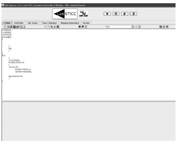
Here, we give a step-by-step account for MemExplorer to obtain a data mapping. The first example is a classical signal processing application called a FIR filter. In this application, we have three data structures to map into the memory hierarchy. Two of them called samples and coefficients are de noted by H and X; the result of the filter is denoted by Y. Each data structure is composed of 1,024 elements of 32 bits each. Structures X and H are accessed at the same time to increase parallelism so if one wants to decrease the conflict cost, one has to map them into two different memory banks. The output Y can be mapped into any memory bank because it is not accessed in parallel with any other data structure. The first step to take in using the MemExplorer tool is to choose the C code to be analyzed. Figure 6.9 shows the edition of the C code for the FIR filter.
Once the C code has been analyzed, a XML file is generated allowing the user to verify if all the codes have been processed (see Figure 6.10).
The next step is to define the MCG; this graph is generated by using the power estimation tab (see Figure 6.11). In this tab, one must choose the C6201 processor (in the future, more processors will be available), the data model for the prediction model (this allows taking into account the data accesses), the frequency (only used for power estimation in SoftExplorer), the mapped memory mode (use of the internal memory bank) and finally a coarse estimation for the prediction tab. Any other configuration will not lead to generating the conflict graph properly.
Figure 6.9. Edition screen
Then, we must choose the initial memory mapping file generated at the same time as the MCG (see Figure 6.12). In fact, the initial memory mapping file considers that all the data structures are in the same memory bank in order to generate the MCG.
The next step is to choose the optimization method that the user wants to use (see Figure 6.13). Four different methods are currently available: a tabu search method, Evocol (these two methods do not take into account the memory size to obtain the best memory mapping, so they are not very useful for this purpose), Vns-TS and finally the integer programming (with GNU Linear Programming Kit (GLPK) solver).
Figure 6.10. XML screen
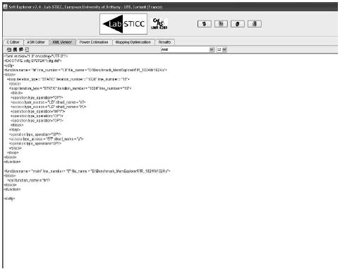
Figure 6.14 shows the result for the FIR filter when Vns-TS is called. We can see that as mentioned at the beginning of this chapter, two data structures of 1,024 elements of 32 bits are stored in memory bank 1 (8,192 bytes of 32,768 bytes), one structure is in bank 0 and thus nothing is in the external memory (named 2 here).
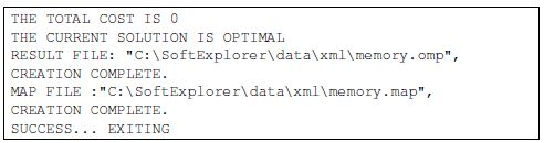
Finally, Figure 6.16 presents the results returned by the GLPK-based method. The solution found with this method shows that our result is optimal and identical to the one returned by Vns-TS.
Figure 6.11. Conflict graph generation screen
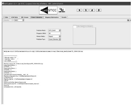
Figure 6.12. Mapping file selection screen
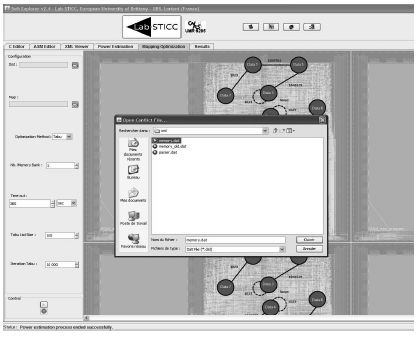
Figure 6.13. Optimization tab screen
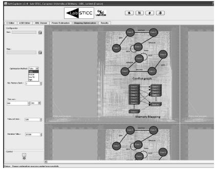
Figure 6.14. Vns-TS mapping optimization screen
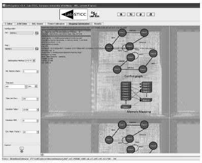
Figure 6.15. Vns-TS mapping optimization Output
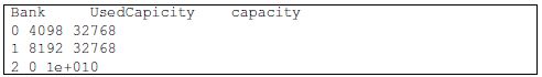
Figure 6.16. GLPK mapping optimization Screen
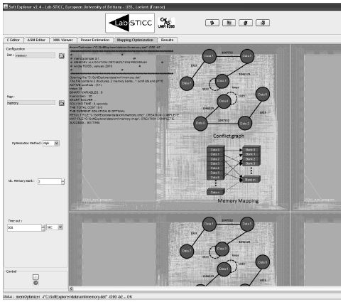
Figure 6.17. GLPK mapping optimization output