Appendix A. Statistical Functions and Tables

The Normal Distribution

For a normally distributed random variable z with mean m and standard deviation σ, the probability that z is less than or equal to some arbitrary value x is given by

(A.1.)

Likewise,

(A.2.)

For any valid probability distribution,

(A.3.)

Therefore,

(A.4.)

The function F_z(x) is a normal or Gaussian probability distribution function. The integrand of c Equation (A.1) is the corresponding probability density function, p_z(α):

(A.5.)

Figure A.1 and Figure A.2 illustrate the probability density and probability distribution functions for a normal random variable with zero mean and unity standard deviation. For this case, the distribution and density functions are

(A.6.)

(A.7.)

Figure A.1. Probability Density Function of a Normal Random Variable

Figure A.2. Probability Distribution Function of a Normal Random Variable

We can obtain a result of the same form as Equation (A.6) by performing a change of variables for Equation (A.1).

Equation (A.6) is similar in form to the error function, erf(y), which has the form

(A.8.)

Note that the erf is odd symmetric about the origin, that is, erf(-y) = -erf(y). Furthermore, erf(∞) = 1 so that erf(-∞) = -1. The simple change of variable yields

(A.9.)

Given its odd symmetry, we can express Equation (A.6) in terms of the erf:

(A.10.)

Simplifying the notation, the normal distribution function, F_z(x), can be expressed in terms of the error function:

(A.11.)

The complementary error function, erfc(y), is defined as 1- erf(y) and can be expressed as

(A.12.)

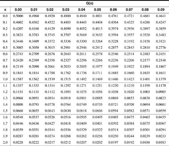
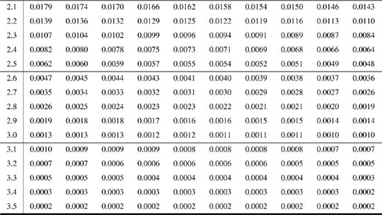
Similarly, the complementary normal distribution function, Q(x), is defined as

(A.13.)

Function Tables

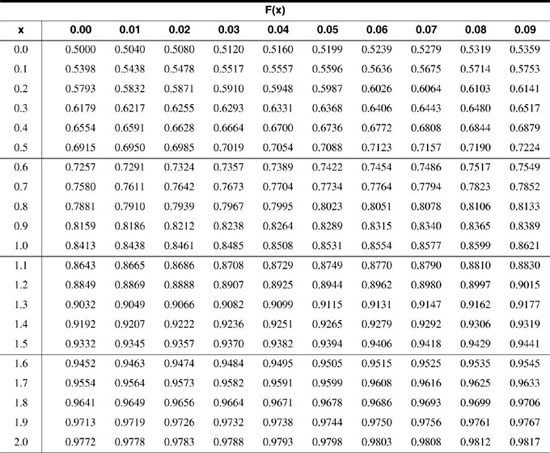
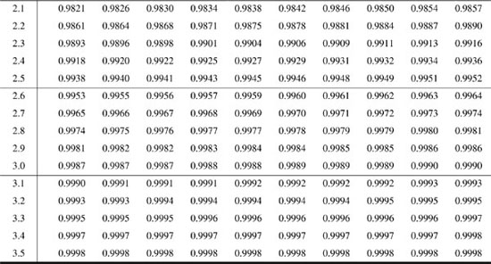
The functions F_z(x) and Q(x) are both integrals of a zero-mean, unity-variance normal probability density function:

(A.14.)

(A.15.)

Tables for both F_z(x) and Q(x) are provided below. When using the tables, F_z(-x) can be evaluated by using Q(x). Similarly, Q(-x) can be evaluated by using F_z(x).

The following MATLAB functions, Ffun(x) and Qfun(x), compute F_z(x) and Q(x). They can be used for both positive and negative values of x.

---

%
% ********** Ffun(x) ***************
%
% This function computes the F-function F(x).
%
function Ffun(x)
sqrt2=sqrt(2);
F=1-0.5*erfc(x/sqrt2)
%

% ************ QFun ***************
%
% This function computes the Q-function Q(x).
%
function Qfun(x)
sqrt2=sqrt(2);
Q=0.5*erfc(x/sqrt2)

---

To evaluate either function for a distribution with mean m and standard deviation σ using the tables, use the forms

(A.16.)

The following MATLAB functions, Ffun2(mean, std_dev, x) and Qfun2(mean, std_dev, x), compute F_z(x - m / σ) and Q(x - m / σ). They can be used for both positive and negative values of x.

---

%
% ********** Ffun2(mean, std_dev,x) ***************
%
% This function computes the F-function F((x-mean)/std_dev)).
%
function Qfun2(mean, std_dev,x)
y=(x-mean)/std_dev;
sqrt2=sqrt(2);
F=1-0.5*erfc(y/sqrt2)
%

% ********** Qfun2(mean, std_dev,x) ***************
%
% This function computes the Q-function Q((x-mean)/std_dev)).
%
function Qfun2(mean, std_dev,x)
y=(x-mean)/std_dev;
sqrt2=sqrt(2);
Q=0.5*erfc(y/sqrt2)

---