Consider a telephone switch that shares K trunks among a large community of users. From time to time, a call from one of the users arrives at the switch, and the switch removes a trunk from the trunk pool and assigns the trunk to the user. From time to time, a call in progress terminates. When this happens the trunk associated with that call is released and is returned to the pool. We can define the state of the switch as the number k of calls in progress at any given moment. Figure B.1 suggests the way the state might vary with time as calls arrive and terminate.
Figure B.1. The State of the Switch
If the switch is in state k = K, then all the trunks are in use and a call arriving at the switch will be blocked. There are two policies for dealing with blocked calls. In the blocked calls cleared policy, the incoming call is shunted to a busy-signal generator. The user must terminate the attempt and may try again later. In the blocked calls delayed policy, the incoming call is held on a queue until an in-progress call terminates and a trunk becomes free. Queued calls are served on a first-come, first-served basis. The blocked calls cleared policy is familiar, as this policy is used by the public switched telephone network. The blocked calls delayed strategy is also familiar as the "please hold for the next available operator" routine used by the customer service departments of many organizations. In this appendix we will consider only the blocked calls cleared policy. The reader is referred to the literature for blocked calls delayed.
The grade of service (GOS) that the switch provides is the probability Pb that an incoming call will be blocked. Telephone systems are typically designed to provide a grade of service of a few percent during the weekly busy hour. We will assume that during the busy hour the average user places λuser calls per minute and holds each call an average of  minutes. Our task in this appendix is to relate the call parameters λuser and , the grade of service Pb, and the number of trunks K to the number N of users that the system can handle. As a result of our analysis we will be able to determine for a given number of users how many trunks will be needed to guarantee any desired grade of service. It should be noted that the call parameters λuser and are empirical parameters that are not produced by a theoretical calculation, but are obtained from measurement and experience.
Whenever a call arrives at the switch, the state of the switch increases by one. For the derivation to follow we will need a statistical model for call arrivals. We will begin with four assumptions.
An arrival process that satisfies these four assumptions is called a "Poisson" process in the literature. It turns out that a Poisson process is an excellent model for call arrivals, especially when there is a large community of users, all of whom act independently. Figure B.2 shows the call arrivals from the example of Figure B.1. It should be noted that the call arrivals include new calls as well as calls that are retries of previously blocked calls. These all look the same to the switch!
Figure B.2. Call Arrivals from Figure B.1

A classical property of Poisson processes, derivable from the assumptions given above, is that if Δt is an arbitrary time interval, not necessarily small, then the probability of k arrivals in Δt seconds is given by
Now suppose we begin observation at some arbitrary time t0, and we wonder how long we will have to wait for the next call to arrive. Let T represent waiting time, and let  be a particular value of T. Then
This expression is the cumulative probability distribution function for the waiting time T. We can find the probability density function for T by differentiating with respect to :
Now let us use this probability density function to find the average waiting time  .
.
This is one way to justify our interpretation of λ as the average number of calls per second. It is interesting, and counterintuitive, to note that the average waiting time does not depend on when we start waiting. The start time t0 is arbitrary and may be the time of the previous call arrival, or not.
Suppose we come upon a call in progress. How much longer will the call continue? Let H represent the remaining duration of the call, known as the holding time. To model the holding time we will take our inspiration from the preceding calculation for the time we must wait for the next call to arrive. The holding time H is modeled as having an exponential distribution
where μ is a parameter to be identified shortly, and η is a dummy variable. Statistics gathered on the duration of actual calls have verified that the exponential distribution is indeed a very accurate model for holding time, with the exception that there are fewer very short calls than the model predicts. It turns out that relatively few calls are shorter than the time it takes to say "Hello."
Given the model in Equation (B.5), we can calculate the average holding time , that is,
This identifies the holding time parameter μ as the reciprocal of the average holding time. As noted previously, average holding time is generally measured in minutes.
In the work to follow we will need to know the probability that a call in progress terminates in a very short interval of time. Suppose δt is such an interval, where δt  . Suppose we begin observing a call in progress at time t0, and we want the probability that the call terminates on or before t0 + δt. Now from Equation (B.5)
where in the last line we have used the Taylor series for the exponential, e-μ
δt  1 - μ
δt for μ
δt 1 or δt .
1 - μ
δt for μ
δt 1 or δt .
Let p(k;t), k = 0,..., K represent the probability that the switch is in state k at time t. We want to consider how these state probabilities evolve in time. As a way to get started, consider what can happen between time t0 and time t0 + δt. In particular, the switch can be in state k = 0 at time t0 + δt in two ways. Either the switch was in state k = 1 at time t0 and the call in progress ended, or the switch was in state k = 0 at time t0 and no new calls arrived. Therefore,
where we have taken the probability that a call in progress ends from Equation (B.7) and the probability that no new calls arrive from assumption 3 of our Poisson model for call arrivals. Rearranging Equation (B.8) gives
If we take the limit as δt → 0, we obtain
where the subscript has been dropped from the time variable in the interest of generality.
Now let us consider how the switch might be in state k = 1 at time t0 + δt. First, the switch might have been in state k = 0 at time t0 and a new call arrived. Remember that the probability that more than one new call arrives in a short interval of time is negligible. Second, the switch might have been in state k = 2 at time t0 and one or the other of the two calls in progress ended. The probability that both calls end is on the order of  and is therefore negligible. Finally, the switch might have been in state k = 1 at time t0 and no new calls arrived and the existing call did not terminate. Putting these possibilities together gives us
Rearranging Equation (B.11) gives

Letting δt → 0 then gives
We can continue this argument state by state. For state k we find
Figure B.3 shows the flow of probability leading to Equation (B.14). For the highest state k = K the results are a little different, as there are only two ways of reaching state k = K at time t0 + δt. We obtain
Figure B.3. How the Switch Can Get into State k at Time t0 + δt
Now suppose we start the switch off in state zero at time zero and let it run (that is, p(0;0) = 1, and p(k;0) = 0 for k = 1,..., K). After a while the solutions to the differential equations given in Equations (B.10), (B.14), and (B.15) will approach steady-state values. Let us call these steady-state probabilities P(k), k = 0,..., K (i.e., P(k) = p(k;∞)). Before we solve for these steady-state probabilities, let us take a moment to discuss what the steady-state probabilities mean. Suppose we have a large number, say 1000, of identical switches that we can operate under identical conditions. Suppose we start them all off in state zero at the same time and let them run. After a long time we come back and examine the switches. At the moment we examine the switches we will find that a certain fraction of them happen to be handling k calls. This fraction is P(k). If we go away and return later, we will find that calls have terminated in some of the switches and new calls have arrived at some of the switches. If we check to see which switches are handling exactly k calls, we may find a somewhat different group of switches from those we identified previously. Nevertheless, the fraction of the total number of switches that have k calls in progress will be about the same, P(k).
Now in the steady state the probabilities p(k;t) are constant with time. This means that the derivatives  will be zero for k = 0,..., K. Our differential equations then become
from Equation (B.10),
from Equation (B.14), and
from Equation (B.15).
Beginning with Equation (B.16) and proceeding iteratively gives, first,

Then from Equation (B.17)
and
and so on. The general term is
which the reader can easily verify by substituting into Equation (B.17). Finally, Equation (B.18) gives
Putting together Equations (B.19), (B.22), and (B.23) gives us
It seems that we would know all of the steady-state probabilities if we only knew P(0). There is one more equation, however, and this will allow us to find P(0) and then all of the P(k). The additional equation represents the fact that the switch must be in some state, that is,

Substituting Equation (B.24) in Equation (B.25) gives
Solving for P(0),
Finally, substituting back into Equation (B.24) gives us the steady-state probabilities that we seek:
We began this derivation with the intent of relating the blocking probability to the call statistics, the number of trunks, and the number of users. The goal is now within sight! If the switch is in state k = K when a call arrives, then the call will be blocked, as all of the trunks will be in use. Thus P[blocking] = Pb = P(K). We can now see from Equation (B.28) that the probability that an arriving call will find the switch in state k = K is
There is now just one loose end to clean up. The parameter λ
that appears in Equation (B.29) is called the offered load and is represented by the symbol A. Offered load is described as a measure of the traffic intensity presented to the switch. It is the product of the average number of calls per unit time arriving at the switch and the average holding time. If λ is measured in calls per minute and is measured in minutes, then A will be a dimensionless quantity. According to tradition, A is given the unit of erlangs after the Danish mathematician Agner Erlang (1878–1929), who initially developed the theory presented here. Now A is the aggregate offered load as seen by the switch. Each user presents an individual offered load given by Auser = λuser
. Recall that λuser is the average number of calls per unit time generated by a single user. We can relate the aggregate offered load to the individual offered load by the simple relation
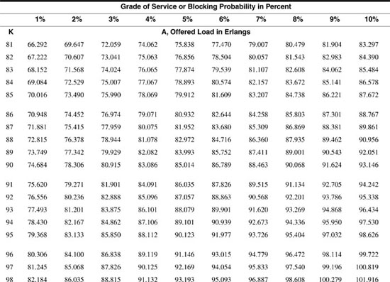
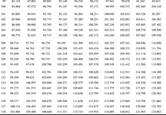
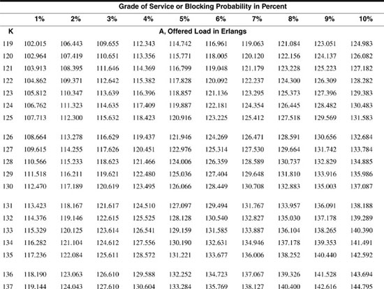
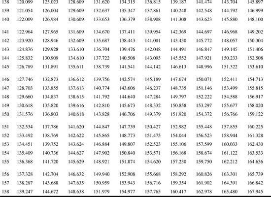
where N is the number of users. Substituting A into Equation (B.29) gives us the result we seek, the celebrated Erlang B formula,
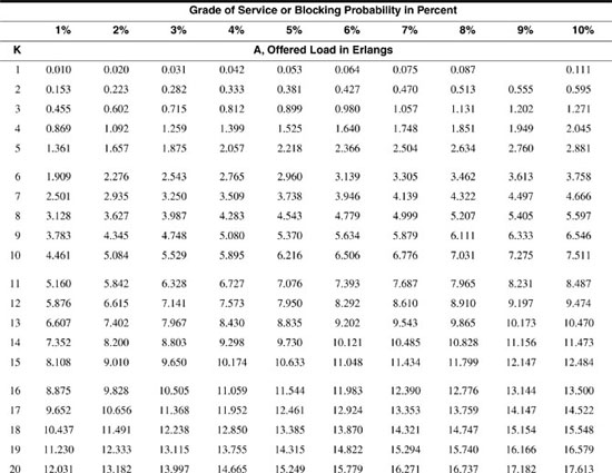
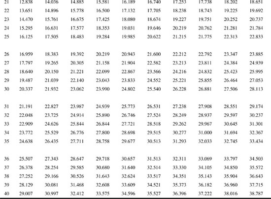
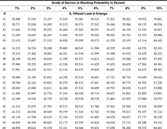
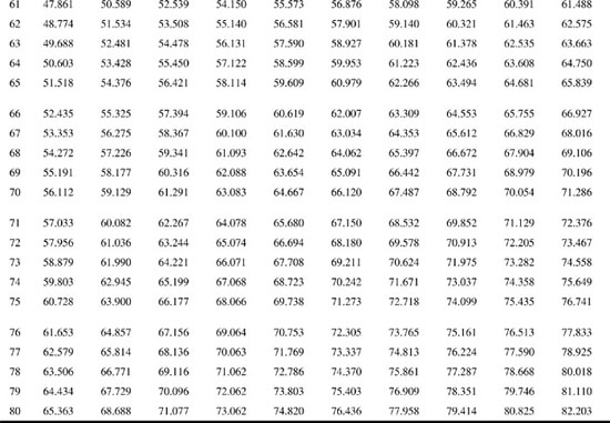
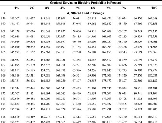
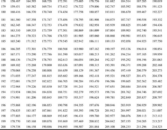
where Pb is the blocking probability, A is the offered load, and K is the number of trunks.
The Erlang B formula contains terms of the form

When evaluating Equation (B.32), the factorial term may exceed the maximum floating-point number that a host computer can support for large values of K. For the computer that was used to generate the tables in this appendix, the upper limit for the factorial term was reached for K = 170. Likewise, the value of AK may exceed the maximum number for large A and K. A typical switching office, however, may possess several thousand serving elements, thereby eliminating the possibility of computation of the GOS by direct evaluation of Equation (B.31). These computational difficulties can be eliminated by a simple rearrangement of the formula.
Starting with the Erlang B formula of Equation (B.31), we divide both numerator and denominator by the numerator. This yields
Reversing the summation so that the terms range from K to 0 and are listed from left to right, we can expand the denominator to obtain

A simple approach to evaluating Den is to form the vector of elements:
Next, compute a vector, prods, containing the cumulative products of the vector ratio such that the nth element is the product of the first n elements of ratio. The vector prods contains the elements
The elements of prods are then summed to form Den.
For A > K the values of the terms decrease from left to right. Therefore, Den converges to a limit for any practical value of K. For K > A the values of the terms increase from left to right. If the ratio K/A is sufficiently large, Den may grow beyond the largest floating-point value that the host computer can support. For most practical situations, however, the ratio K/A and the absolute value of K are such that the limit is not reached. As an example, the largest floating-point number that can be represented by the PC used to generate the tables in this appendix is 1.7977e + 308. For situations that do exceed the maximum floating-point number limit a direct evaluation of Equation (B.31) using the techniques described above can be used effectively.
The following MATLAB function, "Erlangb.m," computes the blocking probability for a given number of servers, K, and offered load, A, in erlangs using the approach described above.
%
% **************** Function "ErlangB" ***************
%
% This function evaluates the Erlang B formula to provide the GOS or
% blocking probability for a specified number of servers, K, and
% an offered load, A.
%
function Pb=ErlangB(A,K)
%
% Ensure that A is positive.
%
if A<0
A=realmin;
end
%
% The numerator of the Erlang B formula contains terms of the form A^K/K!.
% The factorial term is limited to about K=170 depending on the maximum
% positive number that the host computer supports.
% To overcome this limitation we use the approach described in the notes.
%
% Form a vector of length equal to the rounded value K with
% each element value equal to A.
%
AtoK=ones(1,round(K))*A;
%
% Form a vector with element values from the rounded value of K to 1.
%
Kfac=[round(K):-1:1];
%
% Form the vector whose elements are [K/A, (K-1)/A, K-2)/A, ..., 1/A]
%
ratio=Kfac./AtoK;
%
% Augment the ratio vector with a "1" for the i=K term
%
%
ratio=[1 ratio];
%
%
% Form the vector "prods" whose elements are the cumulative products of the
% elements
% of the vector "ratio". The nth element of "prods" is the product of the first
% n elements of "ratio".
%
prods=cumprod(ratio);
%
%
% Add the elements of "prods" one at a time testing the fractional percentage
% change
%
% in the cumulative sum. When the change is smaller than the number of floating-point
% digits carried by the host computer, the summation is ended.
sum=0;
for i=1:K+1
oldsum=sum;
sum=oldsum+prods(i);
delta=prods(i)/sum;
if delta < eps
break
end
end
%
% The blocking probability is the reciprocal of the sum.
%
Pb=1/sum;
The MATLAB routine "GOS" below uses the function "ErlangB" to provide a convenient evaluation tool. The routine requests the number of servers available and the offered traffic to compute the GOS or blocking probability.
% *************** Routine GOS ***********************%
%
% This program computes the grade of service or blocking probability
% for a specified number of servers, K, and a specified offered load, A.
%
% The routine has two loops. The outer loop requests the number of servers
% as an input. The inner loop requests the offered load as an input.
% A blank or negative input breaks either loop.
%
clear
K=realmin;
while K>0
K=input('How many servers are in the system?: ');
A=realmin;
if K<=0
break;
end
while A>0 & K>0
A=input('What is the offered load in Erlangs?: ');
if A>0
Grade_of_Service=ErlangB(A,K)
end
end
end
As its name implies, the routine "Offered_traffic" computes the maximum amount of offered traffic that can be supported by a specified number of servers at a specified GOS. The number of servers and desired GOS are inputs requested by the routine. Since the offered traffic cannot be expressed explicitly in terms of blocking probability and number of servers, this routine does an iterative search to find the value satisfying the input parameters. It uses functions "DeltaPb" and "ErlangB."
%
% *************** Routine "DeltaPb" *********************
%
% This function calculates the difference between a given
% blocking probability and the value returned by "ErlangB".
%
function f=DeltaPb(x)
global K pb
f=pb-ErlangB(x,K);
%
% *************** Routine "Offered_traffic" ************
%
% This routine computes the offered traffic given the GOS
% and the number of servers. Since the Erlang B formula
% cannot be expressed explicitly in terms of the offered
% traffic, A, it uses MATLAB function "fzero" to perform a
% search around an initial guess. It uses functions "DeltaPb"
% and "ErlangB".
%
clear
global K pb
Pb=eps;
opt=[];
while Pb>0
Pb=input('What is the desired GOS in Percent? ');
pb=Pb/100;
K=eps;
A=eps;
while K>0 & Pb>0
K=input('How many servers? ');
if K>0
%
% As an initial guess assume that the offered traffic is
% 90% occupancy.
%
x=.9*K;
%
% Perform a search using the initial guess and the input values
% of Pb and K which are passed to "DeltaPb" using global variables.
% "DeltaPb" is a function that computes the difference between the
% input "Pb" and the value of Pb computed using the initial guess
% for the offered traffic, "x", and the input number of servers, "K".
% "DeltaPb" uses function "ErlangB" to compute each value
% of Pb.
%
A=fzero(@DeltaPb,x)
end
end
end
%
These routines and functions were used to compute the Erlang B tables that follow.
The following provides offered traffic for a range of values for the number of servers and the grade of service.