12
High Performance Liquid Chromatography
- 12.1 Introduction
- 12.2 The Column
- 12.3 Scaling Between Columns
- 12.4 Pumps
- 12.5 Injectors
- 12.6 Detectors
- 12.7 Mobile Phases
- 12.8 Solvents for Sample Preparation
12.1 Introduction
High performance liquid chromatography (HPLC) is a separation technique using high pressure to force the liquid mobile phase through the separation column. The separation column contains small, solid, stationary phase particles. When HPLC was introduced in the late 1960s the name high pressure liquid chromatography was used. Over time, the name was changed to high performance liquid chromatography (HPLC), focusing on the increasingly efficient separations obtained, and common practice is now to use the abbreviation liquid chromatography (LC). Systems capable of running at very high pressures have been introduced in recent years under the name ultra high performance liquid chromatography or ultra high pressure liquid chromatography (UHPLC or UPLC). A schematic overview of an LC system is shown in Figure 12.1.
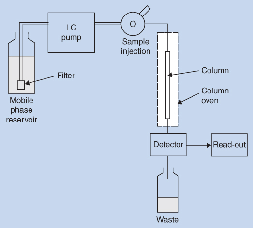
Figure 12.1 Schematic view of LC system
The four main parts of the LC system, the solvent delivery pump (LC pump), the injector, the column, and the detector are all vital and indispensable units. The individual parts of the system are carefully connected by small volume tubing and tight fittings to avoid any dead volumes in the system.
The mobile phase(s) are delivered by the pump and forced with a constant flow rate through the column, which is packed with the column material. The column is often placed in a thermostatic oven (column oven) to control the temperature. Samples are injected to the column by a manual injector or most often by an autosampler. The column may be protected by a short pre‐column. After separation in the column, the individual sample constituents are detected in one or more detectors, which provide an electronic response of the compounds.
The broad applicability and the high degree of automation of LC are among the reasons why this technique has gained such a dominant position in pharmaceutical analysis. LC is used extensively both for chemical analysis of pharmaceutical ingredients and preparations, and for bioanalysis.
12.2 The Column
The column is the heart of the separation process and therefore it is important to keep the column in good condition. The separation columns are typically made of steel tubing and are filled with packing material containing the stationary phase. The packing material is held in place in the column by a filter at each end. The filter is either a porous frit or a net that allows the mobile phase to pass through. The pore size of the filter needs to be smaller than the diameter of the packing material in order to prevent the latter from leaking from the column.
The dynamics of the chromatographic separation process is described by the van Deemter equation. Increasing separation efficiency, expressed by the number of theoretical plates, N, corresponds to the decreasing plate height, and the van Deemter equation describes the theoretical plate height, H, as function of the linear velocity (u). According to this equation, the separation efficiency is highly dependent on the size and uniformity of the particles of the packing material and the separation efficiency is increased when the particle size is reduced. Thus, decreasing the particle size provides a larger number of theoretical plates. This is illustrated in Figure 12.2, showing van Deemter curves plotted for different particle sizes.
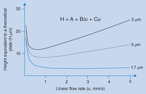
Figure 12.2 Height equivalent to a theoretical plate as a function of the flow rate of the mobile phase for packing materials of different sizes
The van Deemter equation gives several reasons why smaller particles result in narrow peaks. Small particles reduce the different analyte pathways and thereby term A in the equation. At the same time the distance between analyte and stationary phase is reduced for small particles, leading to faster mass transfer of analyte between the phases; this reduces the term C in the equation. The minima of the van Deemter curves (and thereby optimum efficiency) shift towards higher linear flow rates when the particle size is reduced. Thus, higher flow rates can be used without losing efficiency. The practical implication of this is that efficient separations can be achieved on short columns with particles of about 2 μm in a very short time, as shown in Figure 12.3. However, the small particle size also provides a very high back pressure and it may be necessary to use UHPLC equipment.
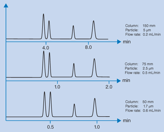
Figure 12.3 LC separation using columns of different packing material size
The typical LC columns used in the European Pharmacopoeia (Ph. Eur.) and the United States Pharmacopeia (USP) are 15–25 cm long, with inner diameters of 4.6 mm, and packed with 5 μm particles. With the introduction of mass spectrometry as a routine LC detection technique and the improvement of column packings, column dimensions of 10–15 cm with a 2 mm internal diameter have become the common standard. For fast UHPLC analysis, smaller particles between 1.5 and 2.0 μm are used in columns of 3–5 cm in length. Using short columns with a small internal diameter result in major savings in consumption of the mobile phase. In Table 12.1, the reduction in mobile phase consumption is calculated for columns of equal length with different internal diameters and operated with the same linear flow of mobile phase. A further reduction of mobile phase consumption is obtained by reducing the column length. A reduction in column length results in a similar reduction in analysis time.
Table 12.1 Saving of mobile phase as a result of the reduction in the internal column diameter keeping the linear flow rate (1.33 mm/s) in the column constant
| Internal diameter (mm) | Flow rate (mL/min) | Reduction in mobile phase (%) |
| 4.6 | 1.0 | — |
| 4.0 | 0.69 | 31 |
| 3.0 | 0.43 | 57 |
| 2.0 | 0.19 | 81 |
| 1.0 | 0.05 | 95 |
Apart from a narrow particle size distribution of the column packing material, low dead volumes of the tubing and connections in the system is important. Tight end fittings of the column and short tubing with a low internal diameter from the injection device to the column and from the column to the detector maintain high quality separations. If non‐optimal connections of tubing and fittings are made during column installation, the separation can be less efficient due to extra band broadening, even if the column itself is in perfect condition. Hence, measuring the efficiency of the ‘column’ is a test of the total system.
12.3 Scaling Between Columns
When operating a LC system, the flow rate of mobile phase is set as volumetric flow as measured in mL/min. In contrast, the van Deemter equation is based on the linear velocity of the mobile phase (u) measured in mm/s. This needs to be considered when changing between columns of different size, and the flow rate and injection volume has to be changed accordingly, as exemplified in Box 12.1. A column with an internal diameter of 4.6 mm is commonly operated with a flow rate of 1 mL/min and an injection volume of 20 μL, while a column with an internal diameter of 2.1 mm is commonly operated with a flow rate of 0.2 mL/min and an injection volume of 5 μL.
12.4 Pumps
Separation and detection occur when the mobile phase is pumped at a constant flow rate through the column. In a standard analytical LC system, the typical flow rate of the mobile phase is 0.2–2.0 mL/min. The small particle size of the column packing materials results in a back‐pressure of 30–300 bar (3–30 MPa) in an LC system and up to 1500 bar (150 MPa) in an UHPLC system, depending on the flow rate. The pumps must therefore be capable of delivering the mobile phase at a constant flow rate against a high back‐pressure. Any particle in the injected samples is trapped on the column inlet and results in gradually blocking the column, which leads to an increased back‐pressure. LC pumps are equipped with a regulation mechanism that keeps the flow rate constant and a gradual blockage thus results in an increase in back pressure while the flow is kept constant.
The pumps deliver the mobile phase at a constant flow rate. The pumps can be constructed in different ways, but a piston pump is the most common and is sketched in Figure 12.4. The piston pump consists of a small steel cylinder with a volume of approximately 100 μL. A piston is moved back and forth in the cylinder by means of a motor. There are two ball valves (check valves) attached to the cylinder so that the mobile phase can only flow in one direction, into the cylinder from the mobile phase reservoir (mobile phase inlet) and out of the cylinder to the LC column. When the piston is moved back the lower ball valve opens while the upper ball valve closes, dragging the mobile phase into the cylinder. When the piston again is moved forward into the cylinder, the bottom ball valve closes while the top valve opens and the mobile phase is forced out of the cylinder and into the LC column. Since the mobile phase is forced into the column only when the plunger is pushed into the cylinder, the flow pulsates. This pulsation introduces extra noise in the detector signal and should be eliminated. A pulse dampener is therefore included in the system to ensure a smooth flow of the mobile phase. Other pump systems ensure a smooth flow by linking together two piston heads into a double piston pump, where one piston head delivers the mobile phase to the column while the second is filled up with the mobile phase.
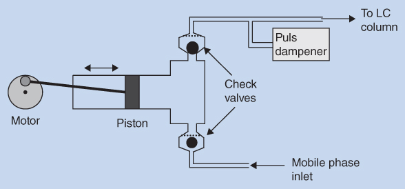
Figure 12.4 Schematic view of a piston pump
When the pumping system delivers a mobile phase with a constant composition to the column, it is called isocratic elution. In a gradient elution system, the composition of the mobile phase is changed during the analytical run. In this case, two mobile phases are pumped from two separate reservoirs and mixed during the analysis. This can be done by low pressure mixing using a single pump equipped with a valve connected to up to four different mobile phase reservoirs. The mixing valve opens for only one pipeline at a time and in this way the solvent mixture can be controlled. Alternatively, high pressure mixing is performed by two pumps, each delivering a controlled amount of mobile phase. The mixing is then performed at the high pressure side. Gradient elution can be compared to temperature programming in gas chromatography (GC).
Gradient elution is used to separate sample constituents with large differences in retention to avoid an unnecessary long analysis time. This is illustrated in Figure 12.5, where the early eluting substances show partially overlapping peaks in the upper chromatogram for isocratic elution, while the most retained substances elute as broad peaks with a long retention time. Using gradient elution (lower chromatogram), the composition of the mobile phase is continuously changed during the analysis, starting with a weak eluting composition of the mobile phase. In this way, the first eluting compounds are adequately retained, and because the eluting strength of the mobile phase is increased during chromatography, the late elution peaks are now eluted faster.
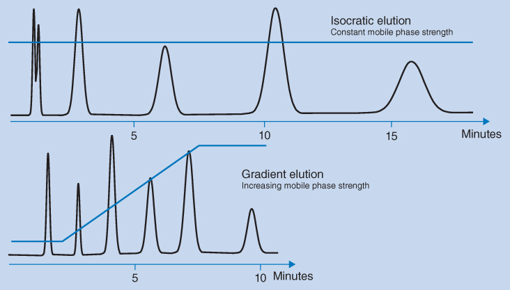
Figure 12.5 Isocratic and gradient elution of a sample containing analytes with large differences in retention
12.5 Injectors
The purpose of the injector is to bring a definite volume of sample solution into the mobile phase and to the column. The substances to be separated must be dissolved in a liquid that is miscible with the mobile phase. In addition, the sample liquid should not have a stronger elution strength than the mobile phase. Typical injection volumes are 5–100 μL. The injection systems are optimized to inject the solution under high pressure and must be leak‐proof in the whole pressure range of the system. For manual injections a simple loop injector as shown in Figure 12.6 can be used.
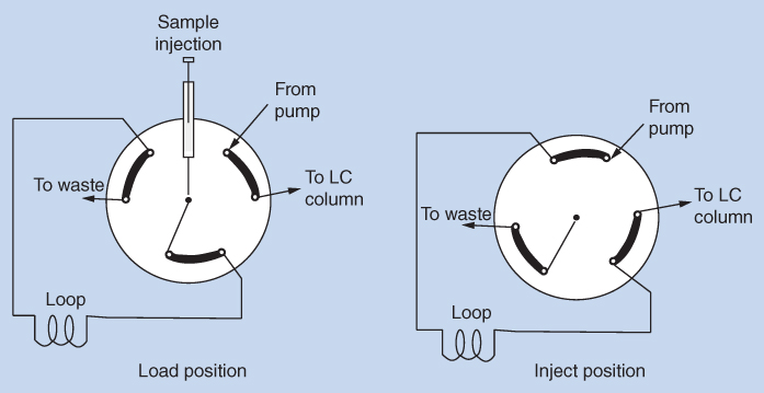
Figure 12.6 Schematic view of a loop injector
The loop injector is a six‐port valve. In the load position the mobile phase from the pump passes through the valve directly to the column. In this position it is possible to inject the sample into the loop using a syringe. When the valve is switched to the inject position, the mobile phase from the pump passes through the loop and in this way brings the sample to the column. The loop is a piece of tubing with a total volume that should not exceed the capacity of the column used. In standard LC systems it is common to use a loop of 20 μL together with columns of 4.6 mm internal diameter. In the load position, the loop is filled with excess sample in order to remove the previous solvent (mobile phase) completely from the loop. After an injection, the injector is switched back to the load position. The channels in the injector are flushed with a cleaning solution between every sample to remove any residual sample solution.
The injection process is most often automated by use of an autosampler. Sample vials are placed in the autosampler and samples are injected automatically into the LC according to pre‐programmed volumes and time intervals. Thus, large series of samples can be analysed automatically. The autosampler is temperature controlled, and sensitive samples can be stored there at a low temperature (typically 5 °C) prior to analysis.
12.6 Detectors
The purpose of the detector is to generate an electrical signal (response) for each compound eluting from the column. The detector response should be proportional to either the concentration or the mass of the compound in such a manner that quantitative analysis can be carried out based on the measurement of peak areas or peak heights. The main LC detectors used in pharmaceutical analysis are given in Table 12.2.
Table 12.2 LC detectors and their typical performance
| Detector | Lower limit of detection (ng) | Gradient elution |
| Ultraviolet (UV) | 0.1–1.0 | Yes |
| Fluorescence | 0.001–0.01 | Yes |
| Electrochemical (ECD) | 0.01–1.0 | No |
| Mass spectrometry (MS) | 0.001–0.01 | Yes |
| Refractive index (RI) | 100–1000 | No |
| Evaporative light scattering (ELSD) | 0.1–1.0 | Yes |
| Charged aerosol (CAD) | 0.1–1.0 | Yes |
For chemical analysis of pharmaceutical ingredients and preparations by LC, the UV detector is standard. Fluorescence detectors and electrochemical detectors (ECDs) show much lower detection limits than the UV detector, but only for selected analytes. The mass spectrometer provides important information on the molecular structure and is a common detector with LC in bioanalysis. LC combined with mass spectrometry is abbreviated LC‐MS and is described in Chapter . A refractive index (RI) detector may be used in case analytes do not absorb UV radiation. It is considerably less sensitive than UV detection and it is not applicable to methods using gradient elution.
12.6.1 UV Detectors
UV detectors are preferred for LC of pharmaceutical ingredients and preparations, mainly due to high operational stability and ease of use. The lower limit of detection is sufficient with pharmaceutical ingredients and preparations, but is insufficient in bioanalysis where drug substances are measured at low concentrations in biological fluids. UV detection can be used for any analyte absorbing UV or visible light. This requires the analyte to contain a chromophore.
According to Beer's law, the absorbance is proportional to the concentration of the substance in the mobile phase, the path length of radiation through the flow cell, and the molar absorption coefficient of the substance. Figure 12.7 shows a sketch of a traditional UV detector for LC.
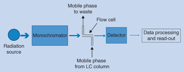
Figure 12.7 Schematic view of a UV detector
The radiation source is most often a deuterium lamp that emits a continuum of light in the UV region (190–400 nm) and any wavelength can be selected by the monochromator. For optimal detection sensitivity, substances should be measured at a wavelength corresponding to their maximum UV absorbance. The mobile phase from the LC column (eluent) passes through a flow cell inside the UV detector and UV light with the selected wavelength is directed through the flow cell where the intensity is measured by a detector (light sensor).
Figure 12.8 shows a sketch of a flow cell. The mobile phase from the column flows through a Z‐shaped channel in the cell. The UV light passes the flow cell through two quartz windows that do not absorb UV radiation. The path length of the flow cell is in the range from 6 to 10 mm, and the volume for a standard flow cell is in the order of 10 μL. Flow cells with a lower volume are available, and these are used when peaks are narrow in order to avoid loss of chromatographic resolution.
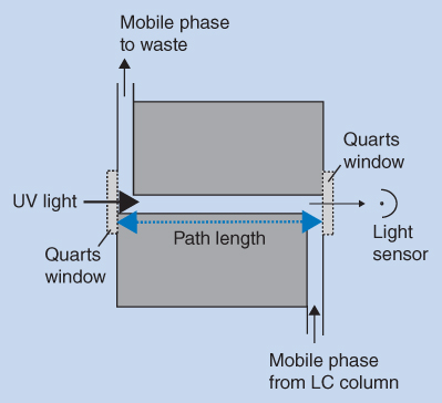
Figure 12.8 Schematic view of the flow cell in a UV detector
Alternatively, UV detection in LC can be accomplished by a diode array detector (DAD), as shown in Figure 12.9. In DADs polychromatic radiation (UV light) is passed through the flow cell. After passage of the flow cell the transmitted light is split in a reflection grating into individual wavelengths and the intensity of each of these is measured by an array of photodiodes (photodiode array). There may be up to several hundred diodes in the array to measure the entire UV region. DADs offer several possibilities. A full UV spectrum of a peak can be recorded during the elution of a given substance and this can be used to identify the substance. An important use of the DAD is for control of peak purity in chromatograms. If the absorption spectrum of a compound changes during the elution of a peak, it is an indication that more than one compound is present in the peak (co‐elution) and separation is not complete.
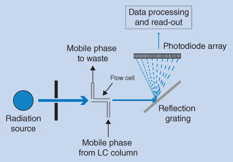
Figure 12.9 Schematic view of a diode array detector (DAD)
12.6.2 Fluorescence Detectors
Some substances emit the temporary energy as fluorescence when they are irradiated. However, while most drug substances absorb radiation in the UV region, only a few substances emit fluorescence. The fluorescence detector is therefore more selective than the UV detector and has lower limits of detection. The detector is therefore useful for detection of low concentrations of fluorescent analytes. In some cases, reaction of analytes with fluorescent reagents and subsequent fluorescence detection is used to improve the sensitivity. Figure 12.10 shows a schematic diagram of a fluorescence detector. The lamp (radiation source) is usually a xenon lamp emitting an intense continuum of light in the whole UV region and partly in the visible region.
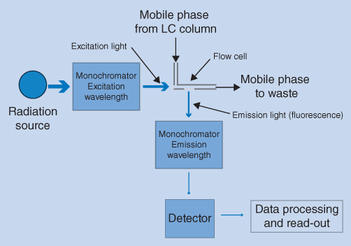
Figure 12.10 Schematic view of a fluorescence detector
The wavelengths of excitation and emission light (fluorescence) are controlled by two monochromators. The molecules are excited using intense excitation light of a selected wavelength (excitation wavelength). Some of the absorbed energy is released as heat, and therefore the emitted light (emission wavelength) is shifted towards longer wavelengths. This is shown in Figure 12.11 for quinine as an example. The excitation wavelength is chosen from the UV absorption spectrum of the compound, preferably at the wavelength of the UV absorption maximum, but for selectivity reasons another wavelength can be chosen. The emission wavelength chosen can be varied as the emission spectrum also covers a range of wavelengths. Fluorescence is emitted in all directions but is normally measured perpendicular (90°) to the excitation radiation to reduce background noise.
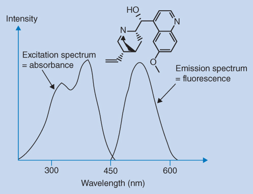
Figure 12.11 Excitation and emission spectra of quinine
For dilute solutions, the following equation expresses how the fluorescence (F) is dependent on a number of parameters:
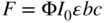
Fluorescence intensity F is proportional to the quantum yield Φ, the intensity of the excitation radiation I0, the molar absorption coefficient of the compound ε, the path length of the detector b, and the concentration of the compound in the mobile phase c. The quantum yield is a compound‐dependent constant in a given environment and describes the fraction of absorbed light that is re‐emitted as fluorescence. As seen from Eq. (12.1), the measured intensity of fluorescence is proportional to the concentration of analyte in the mobile phase. As fluorescence is an emission method, the fluorescence intensity is directly proportional to the intensity of the excitation radiation. Thus, increasing the intensity of the excitation radiation will increase the sensitivity. This is in contrast to absorbance measurements, which are based on the ratio of I0/I. At very low analyte concentrations (low absorption), absorbance measurements are based on two high and almost similar light intensities, while fluorescence is measured on a dark background. Therefore, fluorescence detectors are favourable for detection at low concentration levels.
12.6.3 Electrochemical Detectors
Electrochemical detection is a selective detection principle for compounds with electrochemically active groups that can either be reduced or oxidized, such as phenols, aromatic amines, ketones, aldehydes, and aromatic nitro‐ or halogen‐containing compounds. Oxidation is in practice much easier to perform than reduction because the reduction mode requires that oxygen is totally removed from the mobile phase. The oxidation is performed at a given voltage, typically between +0.3 and +1.0 V. The higher the voltage, the more the substances are oxidized. The detector measures the current as a function of oxidation. The detector is especially well suited for the detection of phenols, amines, and thiols. The ECD is not as robust as UV and fluorescence detectors, and contamination of the electrodes by impurities in the mobile phase and from samples may occur. Pulsed amperometric detection with Au or Pt electrodes expands the applicability of electrochemical detection to cover alcohols and carbohydrates. In this mode, carbohydrates can be detected with high sensitivity, but a high pH value is demanded (pH 12–13), which may not be compatible with the LC system.
12.6.4 Refractive Index, Evaporative Light Scattering, and Charged Aerosol Detectors
The refractive index (RI) detector measures the change in the refractive index of the mobile phase at the column outlet. An analyte with a refractive index different from the mobile phase is detected. However, the detector has low sensitivity and is easily influenced by changes in temperature. In the evaporative light scattering detector (ELSD) the column effluent is nebulized using nitrogen at an elevated temperature. Non‐volatile compounds are detected in the aerosol as they scatter the light from a diode laser. Volatile substances cannot be measured by this technique. The charged aerosol detector (CAD) uses a similar principle for detection. The column effluent is evaporated and an aerosol of non‐volatile compounds is formed. Nitrogen molecules passing a corona receive positive charges that are transferred to the aerosol particles. The positively charged aerosol particles are then measured by an electrometer. Both ELSD and CAD are universal detectors with the exception of volatile substances.
12.7 Mobile Phases
The mobile phases used in LC are contained in bottles, and from there they are withdrawn by the pump through polyethylene tubing, each equipped with a filter that prevents any particles from entering the pump. The following requirements for mobile phase solvents have to be considered:
- The solvents should not give any response in the detector used.
- The solvents must have a satisfactory degree of purity. A number of solvents are available in LC quality and sometimes specified for selected purposes (e.g. for gradient elution or for MS detection).
- The solvents should have low viscosity to provide as low a back pressure as possible in the LC system.
- The solvents should have low toxicity, preferable be inflammable and non‐reactive, and they must be suitable for disposal after use.
Mobile phases for reversed phase LC often contain aqueous buffer solutions. The buffer salts are dissolved in water of LC quality, which is either produced in the laboratory using a water treatment system that removes common contaminants from tap water or obtained commercially. The aqueous solution is mixed with an organic modifier (typically acetonitrile or methanol) to the prescribed solvent strength. If the buffer salts give rise to particles in the solution, it is filtered through a filter with a pore size of 0.45 μm. Before use, the mobile phase has to be degassed to remove dissolved air. Degassing can be performed by ultrasound treatment, by purging with helium, or by vacuum treatment. Vacuum treatment is most common and is now included in most instruments as a continuous online degassing system. Degassing is necessary in order to prevent bubble formation in the detector cell causing noise in the detector signal.
The UV detector is by far the most widely used LC detector. Analytes can be detected when they have a UV response above 195 nm. This requires the mobile phase to be transparent at the given wavelength. Table 12.3 gives an overview of the UV cut‐off of common solvents (organic modifiers). The UV response increases as the wavelength decreases, and the UV cut‐off value is the shortest wavelength that can be used with the solvent.
Table 12.3 UV cut‐off for common solvents (1 cm path length)
| Solvent | UV cut‐off (nm) |
| Acetone | 330 |
| Acetonitrile | 190 |
| Dichloromethane | 220 |
| Ethanol | 210 |
| Heptane | 195 |
| Methanol | 205 |
| Tetrahydrofuran | 210 |
| Water | 190 |
12.8 Solvents for Sample Preparation
A prerequisite for the samples to be analysed by LC is that they are soluble in the mobile phase and the mobile phase is therefore the first choice as a solvent for the sample. In general, the substances should not be dissolved in a solvent with a higher solvent strength than the mobile phase. The use of neat methanol (or acetonitrile) should be avoided in reversed phase LC, as the solvent strength of the sample solution will become too high. If substances dissolved in neat methanol are injected, methanol prevents the substances from being retained on the stationary phase in the column. The substances remain in the methanol plug until it has been diluted with the mobile phase and equilibrium has been re‐established in the system. The result is that the substances are eluted from the column earlier and as broader peaks. If methanol must be used as a solvent, it must be injected only in small volumes in order to prevent peak broadening. If larger sample volumes are to be injected, it is preferable to have a lower solvent strength in the sample compared to the mobile phase. The substances can then under the correct conditions be concentrated at the inlet of the column during the injection, and spreading of extra bands because of dilution in the mobile phase can be avoided.