How to do it...

We will adjust our tables to get the maximum from Redshift in terms of a place for computing, and, allow Tableau to efficiently render the results and visualize it as follows:

1. To choose the right sort key, we should evaluate our queries to find a date column that we are using for filters (the WHERE condition in SQL). For our huge fact table, it is the lo_orderdate column. For the remaining dimension tables, we will use their primary key as a sort key: p_partkey, s_supkey, d_datekey.
2. Then, we will choose candidates for the sort key. The following are the three types of distribution available in Redshift:

• The key distribution
• The all distribution
• The even distribution

You can learn more about Redshift distribution at the following URL:

https://docs.aws.amazon.com/redshift/latest/dg/c_best-practices-best-dist-key.html

3. To find the best distribution style, we need to analyze the SQL query that is generated by Tableau and executed by Redshift. We should use the preceding query to extract the SQL from the cursor. Then, we should look to the execution plan by running our query with the word EXPLAIN, as follows:

explain
SELECT "customer"."c_city" AS "c_city", "dwdate"."d_year" AS "d_year", "supplier"."s_city" AS "s_city",
SUM("lineorder"."lo_revenue") AS "sum_lo_revenue_ok" 
FROM "public"."lineorder" "lineorder" 
INNER JOIN "public"."customer" "customer" ON ("lineorder"."lo_custkey" = "customer"."c_custkey") 
INNER JOIN "public"."supplier" "supplier" ON ("lineorder"."lo_suppkey" = "supplier"."s_suppkey") 
INNER JOIN "public"."dwdate" "dwdate" ON ("lineorder"."lo_orderdate" = "dwdate"."d_datekey") 
WHERE (("customer"."c_city" IN ('UNITED KI1', 'UNITED KI5')) 
AND (("supplier"."s_city" IN ('UNITED KI1', 'UNITED KI5')) 
AND ("dwdate"."d_yearmonth" IN ('Dec1997'))))
GROUP BY 1, 2, 3

We will get the plan as follows:

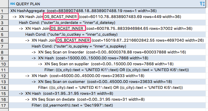
I've highlighted BS_BCAST_INNER. It means that the inner join was broadcasted across all slices. We should eliminate any broadcast and distribution steps. You can learn more about query patterns here:

https://docs.aws.amazon.com/redshift/latest/dg/t_evaluating_query_patterns.html

In our case, we should look at the join between the fact table with 600 mln and dimension tables. Based on fairly small rows in the dimension tables, we can distribute the dimension tables SUPPLIER, PART, and DWDATE across all nodes. For the LINEORDER table, we will use lo_custkey as a distribution key and for the CUSTOMER table, we will use the c_custkey as the distribution key.

4. Next, we should compress our data to make sure that we can reduce storage space, and also, reduce the size of the data that is read from storage. It decreases I/O and improves query performance. By default, all data is uncompressed. You can learn more about compression encodings here: https://docs.aws.amazon.com/redshift/latest/dg/c_Compression_encodings.html. We should use system tables in order to research the best compression encoding. Let's run the following query:

select col, max(blocknum)
from stv_blocklist b, stv_tbl_perm p
where (b.tbl=p.id) and name ='lineorder'
and col < 17
group by name, col
order by col;

It will show us the highest block number for each column in the LINEORDER table. Then, we can start to experiment with different encoding types in order to find the best. In addition, we should always analyze the table after changes in order to update table statistics. However, in our case, we can simply execute the COPY command with the auto compression parameter.

5. Let's apply the changes to our tables and run the same report. Copy the queries from the Create_Statementv2_Redshift.sql file and run them.
6. Then, we should reload data with autocompression. Run SQL from the COPY data to Redshiftv2.txt file. Don't forget to insert your ARN.
7. Let's refresh our Tableau workbook and see the improvements. Moreover, we can check the query plan and see the changes. In my case, it took 8 seconds.