Here’s another chapter of material involving more ways to apply the derivative to several other types of problems. This stuff focuses mainly on using the derivative to aid in graphing a function, etc.
One of the most common applications of the derivative is to find a maximum or minimum value of a function. These values can be called extreme values, optimal values, or critical points. Each of these problems involves the same, very simple principle:
A maximum or a minimum of a function occurs at a point where the derivative of a function is zero, or where the derivative fails to exist.
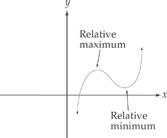
At a point where the first derivative equals zero, the curve has a horizontal tangent line, at which point it could be reaching either a “peak” (maximum) or a “valley” (minimum).
If the derivative of a function is zero at a certain point, it is usually a maximum or minimum—but not always.
There are two different kinds of maxima and minima: relative and absolute. A relative or local maximum or minimum means that the curve has a horizontal tangent line at that point, but it is not the highest or lowest value that the function attains. In the figure to the right, the two indicated points are relative maxima/minima.
There are a few exceptions to every rule. This rule is no different.
An absolute maximum or minimum occurs either at an artificial point or an end point. In the figure below, the two indicated points are absolute maxima/minima. A relative maximum can also be an absolute maximum.

A typical word problem will ask you to find a maximum or a minimum value of a function, as it pertains to a certain situation. Sometimes you’re given the equation; other times, you have to figure it out for yourself. Once you have the equation, you find its derivative and set it equal to zero. The values you get are called critical values. That is, if f′(c) = 0 or f′(c) does not exist, then c is a critical value. Then, test these values to determine whether each value is a maximum or a minimum. The simplest way to do this is with the second derivative test.
If a function has a critical value at x = c, then that value is a relative maximum if f″(c) < 0 and it is a relative minimum if f″(c) > 0.
If the second derivative is also zero at x = c, then the point is neither a maximum nor a minimum but a point of inflection. More about that later.
It’s time to do some examples.
Example 1: Find the minimum value on the curve y = ax2, if a > 0.
Take the derivative and set it equal to zero:
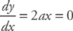
The first derivative is equal to zero at x = 0. By plugging 0 back into the original equation, we can solve for the y-coordinate of the minimum (the y-coordinate is also 0, so the point is at the origin).
In order to determine if this is a maximum or a minimum, take the second derivative:

Because a is positive, the second derivative is positive and the critical point we obtained from the first derivative is a minimum point. Had a been negative, the second derivative would have been negative and a maximum would have occurred at the critical point.
Example 2: A manufacturing company has determined that the total cost of producing an item can be determined from the equation C = 8x2 – 176x + 1800, where x is the number of units that the company makes. How many units should the company manufacture in order to minimize the cost?
Once again, take the derivative of the cost equation and set it equal to zero:
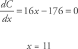
This tells us that 11 is a critical point of the equation. Now we need to figure out if this is a maximum or a minimum using the second derivative:

Since 16 is always positive, any critical value is going to be a minimum. Therefore, the company should manufacture 11 units in order to minimize its cost.
Example 3: A rocket is fired into the air, and its height in meters at any given time t can be calculated using the formula h(t) = 1600 + 196t – 4.9t2. Find the maximum height of the rocket and the time at which it occurs.
Take the derivative and set it equal to zero:

Now we know that 20 is a critical point of the equation. Now use the second derivative test:

This is always negative, so any critical value is a maximum. To determine the maximum height of the rocket, plug t = 20 into the equation:
h(20) = 1600 + 196(20) – 4.9(202) = 3560 meters
The technique is always the same: (a) take the derivative of the equation; (b) set it equal to zero; and (c) use the second derivative test. The hardest part of these word problems is when you have to set up the equation yourself. The following is a classic AP problem:
Example 4: Max wants to make a box with no lid from a rectangular sheet of cardboard that is 18 inches by 24 inches. The box is to be made by cutting a square of side x from each corner of the sheet and folding up the sides (see figure below). Find the value of x that maximizes the volume of the box.

After we cut out the squares of side x and fold up the sides, the dimensions of the box will be:
width: 18 – 2x
length: 24 – 2x
depth: x
Using the formula for the volume of a rectangular prism, we can get an equation for the volume in terms of x:
V = x(18 – 2x)(24 – 2x)
Multiply the terms together (and be careful with your algebra):
V = x(18 – 2x)(24 – 2x) = 4x3 – 84x2 + 432x
Now take the derivative:

Set the derivative equal to zero, and solve for x:
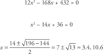
Common sense tells us that you can’t cut out two square pieces that measure 10.6 inches to a side (the sheet’s only 18 inches wide!), so the maximizing value has to be 3.4 inches. Here’s the second derivative test, just to be sure:

At x = 3.4,

So, the volume of the box will be maximized when x = 3.4.
Therefore, the dimensions of the box that maximize the volume are approximately: 11.2 in. × 17.2 in. × 3.4 in.
Sometimes, particularly when the domain of a function is restricted, you have to test the endpoints of the interval as well. This is because the highest or lowest value of a function may be at an endpoint of that interval; the critical value you obtained from the derivative might be just a local maximum or minimum. For the purposes of the AP exam, however, endpoints are considered separate from critical values.
Example 5: Find the absolute maximum and minimum values of y = x3 – x on the interval [–3,3].
Take the derivative and set it equal to zero:

Solve for x:

Test the critical points:

At  , we have a minimum. At
  , we have a maximum.

Now it’s time to check the endpoints of the interval:
At x = –3, y = –24
At x = 3, y = 24
We can see that the function actually has a lower value at x = –3 than at its “minimum” when  . Similarly, the function has a higher value at x = 3 than at its “maximum” of
  . This means that the function has a “local minimum” at
  , and an “absolute minimum” when x = –3. And, the function has a “local maximum” at
  , and an “absolute maximum” at x = 3.
Example 6: A rectangle is to be inscribed in a semicircle with radius 4, with one side on the semicircle’s diameter. What is the largest area this rectangle can have?
Let’s look at this on the coordinate axes. The equation for a circle of radius 4, centered at the origin, is x2 + y2 = 16; a semicircle has the equation 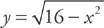 . Our rectangle can then be expressed as a function of x, where the height is
  and the base is 2x. See the figure below:

The area of the rectangle is:  . Let’s take the derivative of the area:
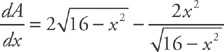
The derivative is not defined at x = ±4. Setting the derivative equal to zero we get:
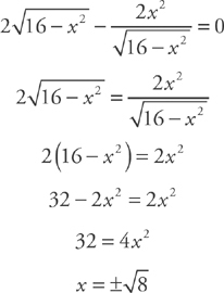
Note that the domain of this function is –4 ≤ x ≤ 4, so these numbers serve as endpoints of the interval. Let’s compare the critical values and the endpoints:
When x = –4, y = 0 and the area is 0.
When x = 4, y = 0 and the area is 0.
When x =  , y = and the area is 16.
Thus, the maximum area occurs when x = and the area equals 16.
Try some of these solved problems on your own. As always, cover the answers as you work.
PROBLEM 1. A rectangular field, bounded on one side by a building, is to be fenced in on the other three sides. If 3,000 feet of fence is to be used, find the dimensions of the largest field that can be fenced in.
Answer: First, let’s make a rough sketch of the situation.
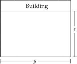
If we call the length of the field y and the width of the field x, the formula for the area of the field becomes:
A = xy
The perimeter of the fencing is equal to the sum of two widths and the length:
2x + y = 3,000
Now, solve this second equation for y:
y = 3,000 – 2x
When you plug this expression into the formula for the area, you get a formula for A in terms of x:
A = x(3,000 – 2x) = 3,000x – 2x2
Next, take the derivative, set it equal to zero, and solve for x:

Let’s check to make sure it’s a maximum. Find the second derivative:

Since we have a negative result, x = 750 is a maximum. Finally, if we plug in x = 750 and solve for y, we find that y = 1,500. The largest field will measure 750 feet by 1,500 feet.
PROBLEM 2. A poster is to contain 100 square inches of picture surrounded by a 4-inch margin at the top and bottom and a 2-inch margin on each side. Find the overall dimensions that will minimize the total area of the poster.
Answer: First, make a sketch.

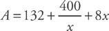
Let the area of the picture be xy = 100. The total area of the poster is A = (x + 4)(y + 8). Then, expand the equation:
A = xy + 4y + 8x + 32
Substitute xy = 100 and y =  into the area equation, and we get:
Now take the derivative and set it equal to zero:

Solving for x, we find that x =  . Now solve for y by plugging x = into the area equation: y = 2. Then check that these dimensions give us a minimum:

This is positive when x is positive, so the minimum area occurs when x = . Thus, the overall dimensions of the poster are 4 + inches by 8 + 2 inches.
PROBLEM 3. An open-top box with a square bottom and rectangular sides is to have a volume of 256 cubic inches. Find the dimensions that require the minimum amount of material.
Answer: First, make a sketch of the situation:

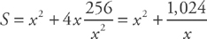
The amount of material necessary to make the box is equal to the surface area:
S = x2 +4xy
The formula for the volume of the box is x2 y = 256.
If we solve the latter equation for y,  , and plug it into the former equation, we get:
Now take the derivative and set it equal to zero:

If we solve this for x, we get x3 = 512 and x = 8. Solving for y, we get y = 4.
Check that these dimensions give us a minimum:

This is positive when x is positive, so the minimum surface area occurs when x = 8. The dimensions of the box should be 8 inches by 8 inches by 4 inches.
PROBLEM 4. Find the point on the curve y =  that is a minimum distance from the point (4, 0).
Answer: First, make that sketch.

D2 = (x – 4)2 + (y – 0)2 = x2 – 8x + 16 + y2
Because y = :
D2 = x2 – 8x + 16 + x = x2 – 7x + 16
Next, let L = D2. We can do this because the minimum value of D2 will occur at the same value of x as the minimum value of D. Therefore, it’s simpler to minimize D2 rather than D (because we won’t have to take a square root!):
L = x2 – 7x + 16
Now take the derivative and set it equal to zero:
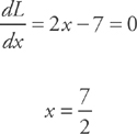
Solving for y, we get  .
.
Finally, because  , the point
  is the minimum distance from the point (4, 0).
Now try these problems on your own. The answers are in Chapter 23.
1. A rectangle has its base on the x-axis and its two upper corners on the parabola y = 12 – x2. What is the largest possible area of the rectangle?
2. An open rectangular box is to be made from a 9 × 12 inch piece of tin by cutting squares of side x inches from the corners and folding up the sides. What should x be to maximize the volume of the box?
3. A 384-square-meter plot of land is to be enclosed by a fence and divided into two equal parts by another fence parallel to one pair of sides. What dimensions of the outer rectangle will minimize the amount of fence used?
4. What is the radius of a cylindrical soda can with volume of 512 cubic inches that will use the minimum material?
5. A swimmer is at a point 500 m from the closest point on a straight shoreline. She needs to reach a cottage located 1800 m down shore from the closest point. If she swims at 4 m/s and she walks at 6 m/s, how far from the cottage should she come ashore so as to arrive at the cottage in the shortest time?
6. Find the closest point on the curve x2 + y2 = 1 to the point (2, 1).
7. A window consists of an open rectangle topped by a semicircle and is to have a perimeter of 288 inches. Find the radius of the semicircle that will maximize the area of the window.
8. The range of a projectile is  , where v0 is its initial velocity, g is the acceleration due to gravity and is a constant, and θ is its firing angle. Find the angle that maximizes the projectile’s range.
9. A computer company determines that its profit equation (in millions of dollars) is given by P = x3 – 48x2 + 720x – 1000, where x is the number of thousands of units of software sold and 0 ≤ x ≤ 40. Optimize the manufacturer’s profit.
Another topic on which students spend a lot of time in calculus is curve sketching. In the old days, whole courses (called “Analytic Geometry”) were devoted to the subject, and students had to master a wide variety of techniques to learn how to sketch a curve accurately.
Fortunately (or unfortunately, depending on your point of view), students no longer need to be as good at analytic geometry. There are two reasons for this: (1) The AP exam tests only a few types of curves; and (2) you can use a graphing calculator. Because of the calculator, you can get an idea of the shape of the curve, and all you need to do is find important points to label the graph. We use calculus to find some of these points.
When it’s time to sketch a curve, we’ll show you a four-part analysis that’ll give you all the information you need.
Find where f(x) = 0. This tells you the function’s x-intercepts (or roots). By setting x = 0, we can determine the y-intercepts. Then, find any horizontal and/or vertical asymptotes.
Find where f′(x) = 0. This tells you the critical points. We can determine whether the curve is rising or falling, as well as where the maxima and minima are. It’s also possible to determine if the curve has any points where it’s nondifferentiable.
Find where f″(x) = 0. This shows you where any points of inflection are. (These are points where the graph of a function changes concavity.) Then we can determine where the graph curves upward and where it curves downward.
Look at what the general shape of the graph will be, based on the values of y for very large values of ±x. Using this analysis, we can always come up with a sketch of a curve.
(1) When f′(x) > 0, the curve is rising; when f′(x) < 0, the curve is falling; when f′(x) = 0, the curve is at a critical point.

(2) When f″(x) > 0, the curve is “concave up”; when f″(x) < 0, the curve is “concave down”; when f″(x) = 0, the curve is at a point of inflection.

(3) The y-coordinates of each critical point are found by plugging the x-value into the original equation.
As always, this stuff will sink in better if we try a few examples.
Example 1: Sketch the equation y = x3 – 12x.
Step 1: Find the x-intercepts:
The curve has x-intercepts at  and (0, 0).
Next, find the y-intercepts:
y = (0)3 – 12(0) = 0
The curve has a y-intercept at (0, 0).
There are no asymptotes, because there’s no place where the curve is undefined (you won’t have asymptotes for curves that are polynomials).
Step 2: Take the derivative of the function to find the critical points:

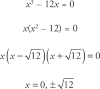
Set the derivative equal to zero and solve for x:
3x2 – 12 = 0
3(x2 – 4) = 0
3(x – 2)(x + 2) = 0
so x = 2, –2
Next, plug x = 2, –2 into the original equation to find the y-coordinates of the critical points:
y = (2)3 – 12(2) = –16
y = (–2)3 – 12(–2) = 16
Thus, we have critical points at (2, –16) and (–2, 16).
Step 3: Now, take the second derivative to find any points of inflection:

This equals zero at x = 0. We already know that when x = 0, y = 0, so the curve has a point of inflection at (0, 0).
Now, plug the critical values into the second derivative to determine whether each is a maximum or a minimum. f″(2) = 6(2) = 12. This is positive, so the curve has a minimum at (2, –16) and the curve is concave up at that point. f″(–2) = 6(–2) = –12. This value is negative, so the curve has a maximum at (–2, 16) and the curve is concave down there.
Armed with this information, we can now plot the graph:

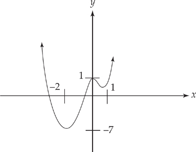
Example 2: Sketch the graph of y = x4 + 2x3 – 2x2 + 1.
Step 1: First let’s find the x-intercepts:
x4 + 2x3 – 2x2 + 1 = 0
If the equation doesn’t factor easily, it’s best not to bother to find the function’s roots. Convenient, huh?
Next, let’s find the y-intercepts:
y = (0)4 + 2(0)3 – 2(0)2 + 1
The curve has a y-intercept at (0, 1).
There are no vertical asymptotes because there is no place where the curve is undefined.
Step 2: Now we take the derivative to find the critical points:

Set the derivative equal to zero:
4x3 + 6x2 – 4x = 0
2x(2x2 + 3x – 2) = 0
2x(2x – 1)(x + 2) = 0
x = 0,  , −2
, −2
Next, plug these three values into the original equation to find the y-coordinates of the critical points. We already know that when x = 0, y = 1.
When 
When x = –2, y = (–2)4 + 2(–2)3 – 2(–2)2 +1 = –7
Thus, we have critical points at (0, 1)  , (−2, −7).
Step 3: Take the second derivative to find any points of inflection:

Set this equal to zero:
12x2 + 12x – 4 = 0
3x2 + 3x – 1 = 0

Therefore, the curve has points of inflection at  .
.
Now, solve for the y-coordinates:
(.26, .90) and (–1.26, –3.66)
We can now plug the critical values into the second derivative to determine whether each is a maximum or a minimum:
12(0)2 + 12(0) – 4 = –4
This is negative, so the curve has a maximum at (0, 1); the curve is concave down there:

This is positive, so the curve has a minimum at  ; the curve is concave up there:
12(–2)2 + 12(–2) – 4 = 20
This is positive, so the curve has a minimum at (–2, –7) and the curve is also concave up there.
If the derivative of a function approaches ∞ from one side of a point and –∞ from the other, and if the function is continuous at that point, then the curve has a “cusp” at that point. In order to find a cusp, you need to look at points where the first derivative is undefined, as well as where it’s zero.
Example 3: Sketch the graph of  .
.
Step 1: Find the x-intercepts:

The x-intercepts are at (±2 , 0).
, 0).
Next, find the y-intercepts:
The curve has a y-intercept at (0, 2).
There are no asymptotes because there is no place where the curve is undefined.
Step 2: Now take the derivative to find the critical points:

What’s next? You guessed it! Set the derivative equal to zero:

There are no values of x for which the equation is zero. But here’s the new stuff to deal with: At x = 0, the derivative is undefined. If we look at the limit as x approaches 0 from both sides, we can determine whether the graph has a cusp.

Therefore, the curve has a cusp at (0, 2).
There aren’t any other critical points. But, we can see that when x < 0, the derivative is positive (which means that the curve is rising to the left of zero); and when x > 0 the derivative is negative (which means that the curve is falling to the right of zero).
Step 3: Now, we take the second derivative to find any points of inflection.

Again, there’s no x value where this is zero. In fact, the second derivative is positive at all values of x except 0. Therefore, the graph is concave up everywhere.
Now it’s time to graph this:

There’s one other type of graph you should know about: a rational function. In order to graph a rational function, you need to know how to find that function’s asymptotes.
A line y = c is a horizontal asymptote of the graph of y = f(x) if:
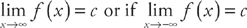
A line x = k is a vertical asymptote of the graph of y = f(x) if:

Example 4: Sketch the graph of  .
.
Step 1: Find the x-intercepts. A fraction can be equal to zero only when its numerator is equal to zero (provided that the denominator is not also zero there). All we have to do is set 3x = 0, and you get x = 0. Thus, the graph has an x-intercept at (0, 0). Note: This is also the y-intercept.
Next, look for asymptotes. The denominator is undefined at x = –2, and if we take the left- and right-hand limits of the function:
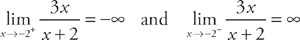
The curve has a vertical asymptote at x = –2.
If we take  and
and 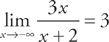 , the curve has a horizontal asymptote at y = 3.
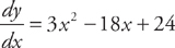
Step 2: Now take the derivative to figure out the critical points:

There are no values of x that make the derivative equal to zero. Because the numerator is 6 and the denominator is squared, the derivative will always be positive (the curve is always rising). You should note that the derivative is undefined at x = –2, but you already know that there’s an asymptote at x = –2, so you don’t need to examine this point further.
Step 3: Now it’s time for the second derivative:
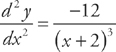
This is never equal to zero. The expression is positive when x < –2, so the graph is concave up when x < –2. The second derivative is negative when x > –2, so it’s concave down when x > –2.
Now plot the graph:

Now it’s time to practice some problems. Do each problem, covering the answer first, then check your answer.
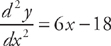
PROBLEM 1. Sketch the graph of y = x3 – 9x2 + 24x – 10. Plot all extrema, points of inflection, and asymptotes.
Answer: Follow the three steps.
First, see if the x-intercepts are easy to find. This is a cubic equation that isn’t easily factored. So skip this step.
Next, find the y-intercepts by setting x = 0.
y = (0)3 – 9(0)2 + 24(0) – 10 = –10
The curve has a y-intercept at (0, –10).
There are no asymptotes, because the curve is a simple polynomial.
Next, find the critical points using the first derivative:
Set the derivative equal to zero and solve for x:
3x2 – 18x + 24 = 0
3(x² – 6x + 8) = 0
3(x – 4)(x – 2) = 0
x = 2, 4
Plug x = 2 and x = 4 into the original equation to find the y-coordinates of the critical points:
When x = 2, y = 10
When x = 4, y = 6
Thus, we have critical points at (2, 10) and (4, 6).
In our third step, the second derivative indicates any points of inflection:
This equals zero at x = 3.
Next, plug x = 3 into the original equation to find the y-coordinates of the point of inflection, which is at (3, 8). Plug the critical values into the second derivative to determine whether each is a maximum or a minimum:
6(2) – 18 = –6
This is negative, so the curve has a maximum at (2, 10), and the curve is concave down there.
6(4) – 18 = 6
This is positive, so the curve has a minimum at (4, 6), and the curve is concave up there.
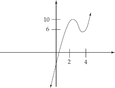
PROBLEM 2. Sketch the graph of y = 8x2 – 16x4. Plot all extrema, points of inflection, and asymptotes.
Answer: Factor the polynomial:
8x2(1 − 2x2) = 0
Solving for x, we get x = 0 (a double root),  , and
, and  .
.
Find the y-intercepts: when x = 0, y = 0.
There are no asymptotes, because the curve is a simple polynomial.
Find the critical points using the first derivative:

Set the derivative equal to zero and solve for x. You get x = 0, x = , and x = −
Next, plug x = 0, x = , and x = − into the original equation to find the y-coordinates of the critical points:
When x = 0, y = 0
When x = , y = 1
When x = −, y = 1
Thus, there are critical points at (0, 0),  , and
, and  .
.
Take the second derivative to find any points of inflection:

This equals zero at  and
and  .
.
Next, plug  and
and  into the original equation to find the y-coordinates of the points of inflection, which are at
  and
and  .
.
Now determine whether the points are maxima or minima.
At x = 0, we have a minimum; the curve is concave up there.
At x = , it’s a maximum, and the curve is concave down.
At x = −, it’s also a maximum (still concave down).
PROBLEM 3. Sketch the graph of  . Plot all extrema, points of inflection, and asymptotes.
Answer: This should seem rather routine by now.
Find the x-intercepts by setting the numerator equal to zero; x = 4. The graph has an x-intercept at (4, 0). (It’s a double root.)
Next, find the y-intercept by plugging in x = 0:

The denominator is undefined at x = –3, so there’s a vertical asymptote at that point.
Look at the limits:
The curve has a horizontal asymptote at y = 1.
It’s time for the first derivative:

The derivative is zero when x = 4, and the derivative is undefined at x = –3. (There’s an asymptote there, so we can ignore the point. If the curve were defined at x = –3, then it would be a critical point, as you’ll see in the next example.)
Now for the second derivative:
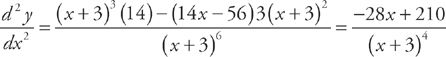
This is zero when x =  . The second derivative is positive (and the graph is concave up) when x < , and it’s negative (and the graph is concave down) when x > .
We can now plug x = 4 into the second derivative. It’s positive there, so (4, 0) is a minimum.
Your graph should look like this:
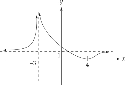
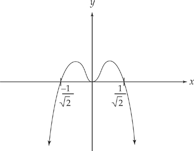
PROBLEM 4. Sketch the graph of  . Plot all extrema, points of inflection, and asymptotes.
Answer: By inspection, the x-intercept is at x = 4.
Next, find the y-intercepts. When x = 0,  .
.
No asymptotes exist because there’s no place where the curve is undefined.
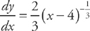
Set it equal to zero:

This can never equal zero. But, at x = 4 the derivative is undefined, so this is a critical point. If you look at the limit as x approaches 4 from both sides, you can see if there’s a cusp:
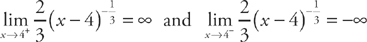
The curve has a cusp at (4, 0).
There were no other critical points. But, we can see that when x > 4, the derivative is positive and the curve is rising; when x < 4 the derivative is negative, and the curve is falling.
The second derivative is:
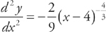
No value of x can set this equal to zero. In fact, the second derivative is negative at all values of x except 4. Therefore, the graph is concave down everywhere.
Your graph should look like this:
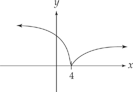
It’s time for you to try some of these on your own. Sketch each of the graphs below and check the answers in Chapter 23.


