Peddlers of visual rubbish know that cherry-picking data is an effective way to deceive people. Choose your numbers carefully according to the point you want to make, then discard whatever may refute it, and you’ll be able to craft a nice chart to serve your needs.
An alternative would be to do the opposite: Rather than display a small amount of mischievously selected data, throw as much as possible into the chart to overwhelm the mental bandwidth of those you want to persuade. If you don’t wish anyone to notice a specific tree, show the entire forest at once.

On December 18, 2017, my day was disrupted by a terrible chart tweeted by the White House. It’s a core tenet of mine that if you want to have cordial and reasonable discussions about thorny issues, you need to use good evidence. The chart, which you can see on the following page, doesn’t fit the bill.
Curious about the chart, I followed the link and saw that it was part of a series against family-based migration. Some graphics pointed out that 70% of U.S. migration in the last decade is family based (people bringing relatives over), which amounts to 9.3 million immigrants.1

I don’t have strong opinions either in favor of or against family-based migration. I’ve heard good arguments on both sides. On one hand, letting immigrants sponsor relatives beyond their closest circle isn’t just a humane thing to do, it also may have psychological and societal benefits; extensive and strong family networks provide protection, security, and stability. On the other hand, it might be a good idea to strengthen merit-based migration and increase the number of highly skilled individuals, in exchange for limiting other kinds of migration.
What I do have strong opinions about are propaganda and misleading charts. First, notice the loaded language, something I warned against in the previous chapter: “chain migration” is a term that has been used widely in the past, but “family-based migration” is much more neutral.
Here’s how the White House describes people moving to the United States: “In the last decade, the U.S. has permanently resettled 9.3 million immigrants solely on the basis of familial ties.” Resettled? I’m an immigrant myself. I was born in Spain, and my wife and children were born in Brazil. We weren’t “resettled by the U.S.” We moved here. And if we ever sponsor relatives, they wouldn’t be “resettled” either; they’d also be moving here voluntarily.
The language the White House used is intended to bias your opinion before you even look at the data. This is a trick that is based on sound science. We human beings form judgments based on quick emotional responses and then use whatever evidence we find to support those opinions, rather than rationally weigh data and then make up our minds. As psychologist Michael Shermer pointed out in his book The Believing Brain, forming beliefs is easy; changing them is hard work.2 If I use charged language, I may surreptitiously trigger an emotional response in my audience that will bias their understanding of the charts.
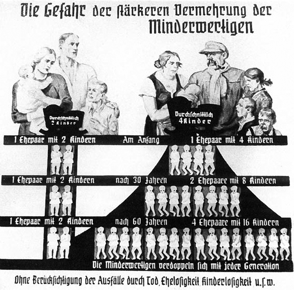
Moreover, the rhetorical style of the White House charts is also tailored to spur emotions. Just see how many new immigrants a single newcomer “has the potential” to spawn! They look like bacteria, vermin, or cockroaches tripling in every generation, a metaphor that has dark historical precedents. The chart the White House tweeted looks eerily similar to charts favored by racists and eugenics proponents. Here’s a German 1930s chart depicting the “danger” of letting the “inferior” races multiply without control:
Charts may lie because they are based on faulty data, but they may also fail because they seem to provide insights while containing no data whatsoever. The White House chart is an example of this.
Who is that prototypical migrant who will end up bringing dozens of relatives? We don’t know. Is that person representative of all migrants? Not at all. Here’s how I know: I arrived in the United States in 2012 with an H-1B visa, reserved for people with specialized skills, sponsored my wife and two kids, and later got a Green Card, becoming a permanent resident. You can think of me as the guy on top of the chart and my family as being on the second step.
So far, so good: me on top, three relatives below me on the chart. The chart is accurate up to that point, although the White House forgot to mention that a majority of the family-based visas assigned every year are for families like mine, made of two spouses and their unmarried children. I don’t think that even the staunchest anti-immigration activist would want to eliminate this policy, although I may be wrong.
But what happens in the lower levels of the chart, when the migrants on the second step start bringing three other relatives each? Well, it’s not that easy: if my wife wanted to bring her mother and siblings, she’d need to sponsor them as non-immediate relatives, a category that excludes extended family such as uncles or cousins. Moreover, to apply for sponsorship in certain visa categories, my wife would need first to become a citizen, so she wouldn’t be a “migrant” anymore.
The number of family-based visas is capped at 480,000 a year. According to the National Immigration Forum, there are no limits on visas for immediate relatives, but this number is subtracted from the 480,000 limit, and therefore the number of visas going to non-immediate relatives is much lower. This means that you can’t bring anyone you want and, moreover, that bringing a non-immediate relative may take years instead, as the number of visas that can go to any one country is limited.
Politically charged topics often yield the best—or worst, depending on your perspective—examples of faulty charts and data. For example, in September 2017, a headline on Breitbart News claimed that “2,139 DACA Recipients Convicted or Accused of Crimes against Americans.”3
DACA stands for Deferred Action for Childhood Arrivals. It’s a policy announced by President Barack Obama in 2012 that protects from deportation some people who were brought to the United States illegally as children and gives them work permits. DACA has many critics who say that it’s a policy created by the executive branch and that it should have been instead discussed in Congress. Some voices I deem reasonable even say it’s unconstitutional,4 and President Trump ended it in September 2017.
This debate is beside the point, though. Let’s focus on the fact that worthy debates can be hindered by flawed graphics. I’ve designed one based on Breitbart’s data point, trying to match the strident rhetorical style of the article:

The first paragraph of the story says:
As Attorney General Jeff Sessions announced the end of the Obama-created Deferred Action for Childhood Arrivals (DACA), from which more than 800,000 un-vetted young illegal aliens have been given protected status and work permits, the number of them who are convicted criminals, gang members, or suspects in crimes remains staggering.
It’s a staggering number indeed, that 2,139.
Not staggeringly high, however, but rather staggeringly low. According to the article, there are more than 800,000 DACA recipients. If that is true, the proportion of them who lost their status for an accusation of being part of a gang or for a criminal conviction is very small.
Let’s do some simple math: If you divide 2,139 by the denominator 800,000, you get roughly 0.003. If you multiply that by 100, you get a percentage: 0.3%. If we multiply by 1,000 instead, we get another rate: out of every 1,000 DACA recipients, 3 lost their status because of their misdeeds.
The number looks even lower if we compare it to something else, which is what we always ought to do. Single figures are meaningless if they aren’t put in context. We could compare that 3 out of 1,000 DACA recipients to a similar proportion of the entire U.S. population. A 2016 study estimates that in 2010 “ex-felons comprise 6.4 percent of the voting age population.”5 That is, 64 over 1,000 people:

My comparison is much more informative than Breitbart’s simplistic article but also imperfect for several reasons: First, this is just one estimate calculated by several scholars (I haven’t, however, managed to find estimates that are significantly smaller). Second, the estimate for the entire U.S. population includes people of all ages. To make a more accurate comparison, we’d need to calculate rates for people who are at most in their thirties, as all DACA recipients are around that age or younger.
Finally, those 3 out of every 1,000 DACA recipients lost their protections not only for felonies but also for misdemeanors and other minor offenses, and the estimate for the entirety of the U.S. population counts only felonies. As the academics who wrote the 2016 study explained:
A felony is a broad categorization, encompassing everything from marijuana possession to homicide. Historically “felony” has been used to distinguish certain “high crimes” or “grave offenses” from less serious, misdemeanor offenses. In the United States, felonies are typically punishable by more than one year in prison, while misdemeanors garner less severe sanctions such as shorter jail sentences, fines, or both.
It may be that if we counted only DACA recipients expelled because of felonies, their number on the chart above would be even lower. We won’t know for sure, however, unless there are more studies.
My first chart based on Breitbart’s data point is an example of a chart that lies because it displays an inadequate amount of data, too little in this case. It also belongs to a subcategory: those charts that, sometimes to help push an agenda, cherry-pick the data and display counts when they should show rates instead, or vice versa.
No chart can ever capture reality in all its richness. However, a chart can be made worse or better depending on its ability to strike a balance between oversimplifying that reality and obscuring it with too much detail. In November 2017, former Speaker of the House Paul Ryan went to social media to promote the Tax Cuts and Jobs Act, a measure passed that same month. He used a graphic like this:

Regardless of what you think of the 2017 tax cut, this graphic is an oversimplification. Averages alone don’t tell you much. How many families in the United States are “average” or close to “average”? A large majority? If I didn’t know better, that’s what I’d think if I trusted Ryan’s figure.
According to the Census Bureau, the median household in the U.S. made $60,000 at the moment of writing this page.6 (Note: Family income may not be the same as household income; a household is one or more people living in the same housing unit, but not all households contain families, which are several people who are related by birth, adoption, or marriage. However, the distributions of family incomes and of household incomes have similar shapes.)
Let’s design a fictional chart that shows that a large majority of households had incomes close to $60,000.

This kind of chart is called a histogram, and it’s used to show frequencies and distributions, in this case, a hypothetical—and false—distribution of U.S. households depending on their income. In this histogram, the height of the bars is proportional to the percentage of households in each income bracket. The taller the bar, the more households there are at that particular income level. Also, if we stacked all the bars on top of each other, they’d add up to 100%.
On my fictional chart, the tallest bars are in the middle, close to the median. In fact, a vast majority of households have incomes between $40,000 and $80,000. The real distribution of household income in the United States is very different, though. Here it is:

The range of household incomes in the U.S. is very wide, spanning from less than $5,000 a year to many millions of dollars. Income distribution is so skewed that we can’t even show it in its entirety on the chart; we need to group wealthy households inside the “$200,000 or more a year” bar. If I tried to keep adding tick marks to the horizontal axis at $5,000 increments, as I did on the rest of the scale, it would extend the chart for dozens of pages.
Therefore, talking just about the average or median family saving $1,182 is nearly meaningless. Most households and families would save either less money or much more than that.
As a taxpayer myself, and as someone who enjoys having civil discussions, I worry about high taxes, but I also worry about balanced budgets and investment in infrastructure, defense, education, and health care. I care about both liberty and fairness. Therefore, I want to know from my representatives how much families all over the income spectrum would save thanks to the tax cut. In a case like this, we must do more than merely refer to a grossly simplified median or average; we must show more data. How much, on average, will people with incomes of $10,000, $100,000, and $1,000,000 save every year?
The Tax Policy Center made the following estimate of the percentage increase in after-tax income that a typical household in each of several income brackets would enjoy thanks to the Tax Cuts and Jobs Act:7
I believe that it’s worth debating whether it’s fair that households making more than $1 million enjoy an increase of after-tax income of 3.3% (3.3% of $1 million is $33,000) while a middle-class family making, say, $70,000 gets an additional 1.6% ($1,120 per year). You’re free to support or oppose the tax cut, but to deliberate about it, we must see data that is much more detailed than a mere average or median.8 These measures of central tendency can be useful, but very often they don’t summarize the shape and texture of a data set well. Charts based on averages alone lie sometimes because those averages capture too little information.

When discussing topics such as income, it is also possible to lie by showing too much information. Imagine that I could plot the income of every single household in the United States, ending up with a chart with tens of millions of little dots. That would, of course, be overkill. We don’t need that level of detail to enable a conversation. The histogram of household income distribution provides a good balance between too much simplification and too much complexity, which is what we should demand from all charts we consume.
I love adventure movies, and Marvel’s Black Panther, directed by Ryan Coogler, is a terrific adventure with a compelling plot and charismatic characters. It was also very successful at the box office, to the point that, according to many news outlets, it became “the third highest-grossing movie of all time in the U.S., behind Star Wars: The Force Awakens and Avatar.”9
This isn’t true. Black Panther was a deserving, smashing success, but it is very likely not the third highest-grossing movie ever in the United States.10
A common problem in stories about movie box offices is that they often contain nonadjusted prices when they should consider adjusted prices. I bet that you’re paying more for goods today than you were five years ago. If you’ve stayed in the same job for many years, your salary may have increased, too. Mine has, but in absolute terms (nominal value), not in relative terms (real value). Because of inflation, even if my salary may look bigger when it enters my bank account every month, it may not feel bigger: the amount of stuff that I can purchase with it is roughly the same as it was three or four years ago.

That’s the challenge behind charts such as the one on the previous page, inspired by data analyst and designer Rody Zakovich,11 who used data from the website Fandango. The chart plots the biggest box office opening weekends (note: Rody is well aware of the chart’s shortcomings).
This chart—which shows first weekend box office records, not total over time, therefore Black Panther isn’t in it—lies in the same way that most of the stories you see in social media touting the latest record-breaking movie lie: they often aren’t adjusted for inflation, so they show nominal values, not real ones. It’s easier to become “the highest-grossing movie” of all time if movie tickets cost $15 instead of $5, in unadjusted dollars. That’s why in many rankings of movie box office, very recent movies are usually on top and older ones are at the bottom.
To correct for this, I converted each movie’s box office in the chart into 2018 dollars using a free online tool created by the Bureau of Labor Statistics.12 I then plotted the results, which look a bit different from the above chart. The ranking of first-week box offices doesn’t change much, but older movies look much better. See for yourself:

In the chart, I compare the unadjusted figures (red line) with the ones adjusted to 2018 dollars. All bars increase in height, but at very different rates: for Star Wars: The Force Awakens (2015), the box office changes by roughly 5%, whereas for Jaws (1975) it grows by more than 360%, which means that if it were released in 2018 it would make not its nominal box office of $7 million but $32 million.
I’m no expert in the economics of film production, just someone who enjoys movies and news, but as a professor and designer who studies charts for a living, I do find that charts and stories discussing successes and flops at the box office tend to be lacking. Isn’t comparing Jaws with The Force Awakens unfair if we don’t consider how much the movie industry has changed? And what about factors such as marketing and promotion efforts, the number of theaters in which each movie opened, and so forth?
I can’t answer those questions, but I can use publicly available data to calculate how much each of the movies above made per theater during its opening weekend, and then I can transform the results into 2018 dollars:

This made me wonder what would have happened if Jaws, which in 1975 opened in 409 theaters in the United States, had instead been released in 2015 in as many theaters as The Force Awakens (4,134)? Would releasing it in 10 times as many theaters have resulted in 10 times its nominal opening weekend box office, moving from $32 million to $320 million? Who knows? It could also be that modern movie theaters have smaller capacities, on average, than the ones in the 1970s. So many questions!
Other metrics of relative success would be profit (the difference between a movie budget and its total box office) and return on investment (the ratio between a movie’s profit and its budget). Movies such as Avatar, The Avengers, and The Force Awakens were very profitable but at relatively high risk, as they cost a lot to produce and to promote. Some estimates say that nowadays you may need to spend as much on marketing as you do on making the movie itself. A 2012 movie designed to be a blockbuster, John Carter, cost Disney more than $300 million to make and market, yet it recovered just two-thirds of that.13
Other movies are much less risky: The movie with the highest return on investment of all time, according to some sources,14 is Paranormal Activity. It made nearly $200 million but it cost only $15,000 to make (marketing costs excluded). Which movie is more successful, Avatar or Paranormal Activity? It depends on the metric we choose and on how we weigh returns versus possible risk on each investment.
Therefore, here’s a new version of my chart. I calculated how much of each movie’s budget—not counting marketing cost—was recovered during its first weekend:

Jaws recovered its entire budget on the first weekend, while other movies made a profit at the outset. The most extreme case is a movie that made twice its entire budget at its opening: Every Which Way but Loose, in which Clint Eastwood partners up with an orangutan called Clyde. Now that I think of it, I loved that movie when I was a kid.
When it comes to designing a chart, which values are better, nominal (nonadjusted) or real (adjusted)? It depends. Sometimes, adjusted values matter much more. Comparing box offices or any other kind of price, cost, or salary over time doesn’t make sense if you don’t adjust your figures, as we’ve just seen. To understand a nominator, you need to pay attention to the denominator, particularly if you make comparisons between groups that have different denominators.
Imagine that I give you two slices from one pizza and I give another person three slices from a different pizza. Am I being mean to you? It depends on how many slices each of the pizzas is divided into:

Not taking denominators into account can have grave consequences. Here’s a bar graph inspired by fictional data provided by Judea Pearl in his The Book of Why: The New Science of Cause and Effect:

Pearl’s fictional data reflects numbers thrown around during heated debates in the 19th century, when the smallpox vaccine became widespread, between those in favor of universal inoculation and those opposed. The latter were worried because the vaccine caused reactions in some children and those reactions sometimes led to deaths.
As alarming as it looks (“More children died because of the vaccine!”), the chart I designed isn’t enough to help you make a decision about whether to vaccinate your own children. For it to tell the truth, I need it to display much more data, including the denominators. This flow and bubble chart can make us smarter at reasoning about this case:

Let’s verbalize what the chart reveals: 99% of children out of my fictional population of 1 million took the vaccine. The probability of having a reaction is roughly 1% (that’s 9,900 out of 1 million). The probability of dying if you have a reaction is also 1% (99 out of 9,900). But the probability of dying because of the vaccine is just 0.01% (99 out of 990,000 who were inoculated).
On the other hand, if you don’t take the vaccine, there’s a 2% probability of getting smallpox (200 out of 10,000). And if you do get the disease, there’s a 20% chance that you’ll die (40 out of 200). The reason why my first chart shows that many more children died because of a reaction to the vaccine than because of smallpox itself is simply that the population that took the vaccine (990,000) is enormously larger than the population of children who didn’t (10,000), a fact that I should have disclosed.
I agree that 99 versus 40 still looks like a huge difference, but try to reason with a hypothetical. Imagine that no children were inoculated against smallpox. We know that 2% will get the disease. That’s 20,000 children out of a population of 1 million. Of those, 20% will die: 4,000 in total. Here’s my updated chart:

The 139 there is the result of adding the 40 kids who weren’t vaccinated and died of smallpox and the 99 who were vaccinated and died after a reaction to the vaccine. The comparison between universal inoculation and no inoculation at all is now more truthfully revealed.
In many cases, both the nominal and the adjusted values matter for different reasons. 100 People (https://www.100people.org/) is a wonderful website that translates many public health indicators into percentages. Out of every 100 people in the world, 25% are children, 22% are overweight, and 60% are of Asian origin. Here’s a statistic that made me feel optimistic:

Data analyst Athan Mavrantonis pointed out that these numbers could be interpreted in a different way:

Which chart is better? The answer is neither. Both are relevant. It’s true that the proportion of people suffering from starvation is small in relative terms—and it keeps shrinking—but it’s also true that behind that 1% figure, there are 74 million human beings. This is a bit less than the population of Turkey or Germany and roughly equivalent to one-quarter of the population of the United States. Now the chart doesn’t look so bright, does it?
Several recent books cast a positive light on human progress. Hans Rosling’s Factfulness and Steven Pinker’s The Better Angels of Our Nature and Enlightenment Now contain an impressive array of statistics and charts corroborating that the world is indeed becoming a better place.15 These books, and the websites they extract their data from, such as Our World in Data (https://ourworldindata.org), suggest that we may soon fulfill the United Nations’ 2015 Global Goals initiative, which aims to “end poverty, fight inequality and stop climate change” by 2030. I do believe that charts like these, based on data from the World Bank, are fabulous news:

In 1981, around 4 out of 10 people in the world had to survive on the equivalent of less than two dollars per day. In 2013, that number dropped to 1 out of 10 people. In 1990, 65 children out of 1,000 died before reaching one year of age. In 2017, that number had dropped to 31.
This is a success story that must be celebrated. Whatever it is that institutions such as the United Nations, UNICEF, and many others are doing in collaboration with governments and nongovernmental organizations, it seems to be working, and it needs to continue.
However, charts and data like these may obscure the massive amount of human misery that hides behind the figures. Percentages and rates numb our empathy. A figure like 10.9% sounds small until you realize how many people it represents—close to 800 million in 2013:

I think that seeing percentages and rates alone (“10.9% of the world population”) when discussing human progress may make us too complacent, as it dehumanizes the statistics. I’m not alone in this hunch. Psychologist Gerd Gigerenzer, author of Calculated Risks, says that percentages make numbers more abstract than they should be. I’d suggest peeking into the raw counts, too, and reminding ourselves that “that’s 783 million people!”
Neither the adjusted figures nor the nominal ones are enough if presented on their own. When shown together, they give us a richer understanding of the breathtaking progress we’ve made—and of the breathtaking challenges we still face. Nearly 800 million human beings in extreme poverty is the equivalent of two and a half times the population of the United States in 2016. That’s a lot of suffering.
Many charts conceal relevant baselines or counterfactuals that, if revealed, would reverse an intended message. Take this 2017 tweet from WikiLeaks founder Julian Assange, accusing modernity of making advanced nations childless and more reliant on immigration:
Capitalism+atheism+feminism = sterility = migration. EU birthrate = 1.6. Replacement = 2.1. Merkel, May, Macron, Gentiloni all childless.16
The leaders Assange mentioned are Angela Merkel, chancellor of Germany; Theresa May, the British prime minister; Emmanuel Macron, president of France; and Paolo Gentiloni, Italy’s prime minister.
Assange illustrated his tweet with a table of data from more than 30 European countries. These are Assange’s figures, in a chart that is as cluttered as the table itself:

Assange made several mistakes. First, he wrote “birth rate,” but the figures he used are fertility rates; the variables are somewhat related, but they aren’t the same. The birth rate is the number of live births per 1,000 people in a country and year. The fertility rate is, to simplify a bit, the average number of children a woman could give birth to during her lifetime. If half the women in a country have 2 children, and the other half have 3, then the fertility rate of that country would be 2.5.
But let’s ignore this mistake and assume that Assange wanted to write “fertility rate.” With his tweet and data display he argued that the fertility rate in these capitalist and secular democracies is quite low—1.6 children per woman on average—and that the leaders of such countries may have something to do with the fact that this figure is far from the minimum fertility rate needed to keep a population stable in the long term, 2.1 children per woman—also called the replacement rate.
Assange’s table and my chart version are spectacular because they accomplish two opposite feats: they lie by showing too little data and too much data—or at least, too much data that hinders rather than enables understanding.
Let’s begin with the latter. Tables with many numbers and charts in which all the lines overlap so much, like mine, make it very hard to extract patterns from the data or to focus on specific cases that may refute our initial opinion. For instance, northwestern European countries tend to be quite secular and favor gender equality. Have their fertility rates dropped dramatically?
We could separate the lines, rather than cram them all into a single chart, and see what happens, on the facing page.
See Denmark or Finland. Their lines display very little variation since 1990, and they stay quite close to the replacement rate of 2.1. Now focus on more religious countries, such as Poland and Albania: the drops in their fertility rates are quite pronounced. Next, notice countries where a majority of the population claims to be Christian, such as Spain and Portugal. Their fertility rates are very far from the replacement rate.
This leads me to guess that the main factor driving changes in fertility rates in countries that have not experienced recent wars or catastrophes might not be religion or feminism, Assange suggested, but perhaps the stability of their economies and societal structures. For instance, unemployment in southwestern European countries such as Spain, Italy, or Portugal has been historically high, and salaries are low; people may delay or abandon the decision to have children simply because they know they can’t afford them. The large drops in some ex-Soviet countries such as Albania, Hungary, Latvia, or Poland in the early 1990s could be related to the fall of the Soviet Union in 1991 and the transition to capitalism.

Migration, as Assange seems to point out in his tweet, might help to increase fertility rates or make a country age more slowly, but to reach that conclusion we need more evidence. Assange’s table and my corresponding charts fail by not showing enough data and context. We are cherry-picking. Fertility rates have dropped not only in secular nations but nearly everywhere in the world, in religious and secular countries alike.

Let’s end this chapter by circling back to the discussion about nominal values and unadjusted data versus rates and percentages. Did you know that the most obese places in the United States are Los Angeles County (California), Cook County (Illinois), and Harris County (Texas)?

Coincidentally, those places are also the poorest in the nation:

The relationship is remarkable—except that it truly isn’t. Here’s a map of county population:

The number of obese people is strongly correlated to the number of poor people simply because both variables are also strongly correlated to the size of the underlying populations: Cook County is where the city of Chicago is, and Harris County contains Houston. Here are two maps with the figures transformed into percentages:

The picture changes quite a lot, doesn’t it? There’s still a vague relationship between obesity and poverty but it’s much weaker, and counties such as Los Angeles are certainly not among the top counties. Los Angeles has so many poor and obese people because it has a big population. Maps that use shades of color to represent data—“choropleth” maps, from the Greek words khōra (place) and plēthos (crowd or multitude)—work better when they display adjusted data, such as percentages of obese and poor people, not raw counts. When they show raw counts they simply reflect the size of the population in the regions they depict.
We can visualize the numbers in a different way, as scatter plots. The first chart on the opposite page shows the relationship between obesity and poverty without adjusting by population; the second one shows the relationship between the percentage of people who are obese and the percentage of people who are poor. (See the charts on the next page.)
Claiborne County, in Mississippi, has the highest percentage of obese people (48% of its 9,000 inhabitants) and Oglala Lakota County, in South Dakota, has the highest percentage of people living in poverty (52% of its 13,000 inhabitants). Los Angeles County, Cook County, and Harris County have obesity rates of between 21% and 27% and poverty rates of between 17% and 19%. They are in the lower-left quadrant of the second chart.
This would be one case where both unadjusted and adjusted figures matter; after all, there are nearly two million poor people in Los Angeles County. But if your goal is to compare counties, the adjusted figures are necessary.
