Chapter 11

Applying RSM to Mixtures

If your experiment needs statistics, then you ought to have done a better experiment.

Ernest Rutherford

Nobel Prize for chemistry 1908

The attitude of elite chemists toward statistics has not improved much from when Rutherford made this insulting statement. Perhaps, the reason is that the standard methods for the DOE don’t work very well on mixtures. For example, let’s say you get a new ultra-high-shear blender and start tossing in various fruits to see if you can make a tasty “smoothie” drink. Table 11.1 shows the experimental layout for a fanciful concoction that might be branded “BanApple.” Is this a good design?

Aside from the dubious choice of ingredients for this mixture design, it makes no sense when you consider that the taste will be simply a function of the proportions of ingredients. Notice that standard orders 1 and 4 end up being the same in terms of the fractions for each fruit. In other words, all that’s been done is a scale-up of the same recipe. Yuk! Who would want to double the dose of a BanApple smoothie? The total amount varies, but will have no effect on responses such as taste, color, or viscosity. Therefore, it makes no sense to do the complete design. When responses depend only on proportions and not the amount of ingredients, factorial designs don’t work very well. The same problems occur with RSM, such as the CCD, which uses factorials as its core.

Table 11.1  Bad Factorial Design on Mixture of Fruit for a “Smoothie”

Std Order	A: Apples	B: Bananas	Proportions (A/B)	Fraction (A, B)
1	2	1	2/1	(0.667, 0.333)
2	4	1	4/1	(0.8, 0.2)
3	2	2	1/1	(0.5, 0.5)
4	4	2	2/1	(0.667, 0.333)

A MIXTURE BY ANY OTHER NAME BEHAVES THE SAME

Mixtures don’t necessarily refer only to physical substances. For example, varying effects can be produced by changing the mix of words in a paragraph. However, writers such as William Safire of the New York Times, who pride themselves on their command of the English language, find the word mixture lifeless. They prefer the word farrago (pronounced fuh-RAY-go or fuh-RAH-go). Farrago, which comes from a Latin word referring to a mixed grain used for making mush (yum!), is synonymous with gallimaufry derived from Old French. However, farrago is as far as we will go into the realm of the esoteric vocabulary for the erudite experimenter.

…what we have been treated to is a farrago of half-truths, assertions and over-the-top spin.

Peter Kilfoyle

Former British Labor Minister

William Safire column “On Language” in The New York Times Magazine, April 27, 2003, p. 22

Accounting for Proportional Effects by Creating Ratios of Ingredients

To many formulators, the ratios of components mean more than the proportions. For example, in the manufacturing of glass, the ratio of silica to alkali has long been considered to be a key factor for product performance (Sullivan and Taylor, 1919). Similarly, the quality of bread dough greatly depends on the flour-to-water ratio (Veal and Mackey, 2000). By converting multiple components into various ratios, experiments involving formulation can then be run using factorial, central composite, or other process designs. In other words, you can mix your cake and bake it too! However, as we will detail, there are downsides to this approach for the mixture design:

  It takes some mathematical finagling to develop ratios that will not violate the constraint that ingredients add up to a fixed total, for example, 100%

  This mathematical finagling must be undone to back calculate from the ratios laid out in the design matrix to actual levels of ingredients (more math ☹)

  The layout of design points in ratio space often translates into a poorly spaced set of formulations.

GETTING A GRIP ON A SLIPPERY FORMULA

In 1953, while trying to develop a missile-part degreaser, rocket chemical technicians made 39 formulations, none of which worked. But number 40 worked like a charm so that they named their product WD-40 as an abbreviation for “water displacement,” perfected on the “40th” try. Noticing that employees started sneaking it home for personal use, the company started selling it to consumers. Over the years, WD-40 has been put to many uses, but none of them have been so unusual; at least, that’s been publicized, as the time that firemen needed it to extract a nude burglar from an air vent. The methods used to develop WD-40 and experiments on how it might be put to the best use remain largely unknown, probably for the better.

www.WD40.com

First of all, let’s address the issue of forming proper ratios. This will not be a problem if you wish to experiment on only two ingredients. For example, it’s not a big deal to make a variety of BanApple smoothies at varying ratios of bananas to apples. An erstwhile entrepreneur could add processing factors, such as blender speed, and create a response surface design aimed at optimizing consumer response. Who knows, maybe, people prefer smoothies that are somewhat lumpy! However, as soon as you add a third ingredient (how about something with some tartness, such as clementines!), the setup of proper ratios starts getting complicated. We must follow certain rules for doing this:

1.  The number of ratios (n_r) is equal to q − 1, where q represents the number of ingredients (or components in the jargon of the mixture design)

2.  Each ratio in the set must contain at least one of the components used in at least one of the other ratios belonging to the set

This latter rule allows the total constraint (often 100%) to be maintained (take our word on this!). Here are several feasible ratios (R_i) for three ingredients (A, B, and C):

  R₁ = A/C, R₂ = B/C

  R₁ = A/B, R₂ = B/C

  R₁ = A/(B + C), R₂ = B/C

Which of these makes most sense entirely depends on the application and what’s been already established as a common practice. This is likely to depend on the chemistry of the formulation. If you really do not care in one way or another, consider labeling the components in a descending order of concentration and then applying the first set of ratios (R₁:A/C and R₂:B/C). This protocol produces ratios greater than one, which you may find more convenient to apply for experimental purposes. For example, in our BanApple smoothie with clementines, assume that we want more apple (A) than banana (B), with clementines (C) being the least of all three ingredients. Then, for purposes of experimentation, two ratios, R₁ (A/C) and R₂ (B/C), could be varied over two levels from low to high. We won’t try quantifying this hypothetical DOE because, as you will see in the next example, it requires some arithmetic.

DON’T LIKE OUR BANAPPLE IDEA? HOW ABOUT A FUZZY BANANA NAVEL!

Try this recipe for a soothing sipper:

  Two medium, ripe DOLE bananas, quartered

  One pint DOLE orange sorbet or two cups of orange sherbet, slightly softened

  One cup DOLE mandarin tangerine juice

Combine bananas, sorbet, and juice in a blender or food processor. Blend until it is thick and smooth. It takes only 5 minutes to prepare and serves four with delicious drinks containing 220 calories, 2 grams of fat (1 gram saturated), 5 milligrams of cholesterol, 38 milligrams of sodium, 1 gram of carbohydrate, and 2 grams of protein.

Do you care to venture a guess as to the source of this recipe? (Hint: It’s a company that was founded in Hawaii in 1851. They are now the world’s largest producer and marketer of high-quality fresh fruit.)

Now, we are ready to illustrate the use of ratios in RSM on an entirely different (not a beverage!) example—blending gasoline (Cornell, 2002, p. 307). A refinery produces three components (q = 3) for automotive fuel. Their ratios of interest are C/A and C/B, respectively. These two ratios satisfy the two rules for feasibility, that is,

1.  Number of ratios n_r = q–1 = 3–1 = 2

2.  One common component in both ratios: C

The blending operation currently operates at ratios:

  R₁ = C/A = 1

  R₂ = C/B = 2

This translates to an actual composition in weight fraction for A, B, and C of 0.4, 0.2, and 0.4. The fuel formulators want to vary each ingredient within the following individual constraints:

A.  0.25–0.60

B.  0.1–0.4

C.  0.2–0.6

The weight fractions for three components must always sum to a total of 1. We mustn’t forget this!

For purposes of optimization, the petroleum chemist responsible for the gasoline product development creates a full three-level factorial design (3²) based on the following ratios:

  R₁ (C/A) = 0.5, 1.0, and 1.5, versus

  R₂ (C/B) = 1, 2, and 3

Notice that these ranges go somewhat below and above the current ratios of ingredients. However, will they conform to the individual component (A, B, and C) constraints? We can answer this vital question by laying out the design on a trilinear graph paper, also known as “ternary” diagrams.

“TURNARY” DIAGRAMS

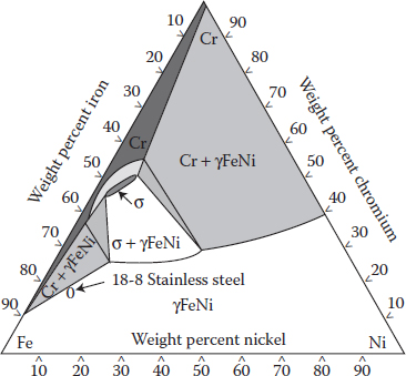
If you are not a chemist, chemical engineer, material scientist, or the like, you may not be familiar with trilinear graph paper. This is a useful tool for metallurgists for diagramming the various phases for alloys such as those shown in Figure 11.1 for stainless steels produced at 900 degrees Celsius (American Society for Metals, 1992).

The three main components of stainless steel are iron (Fe), chromium (Cr), and nickel (Ni). They can be varied from zero at each side of the triangle to 100% of the total weight at the opposing vertices. The most common type of stainless steel, often used for kitchen flatware, is the one pointed out on the graph: 18-8. Its name reflects the composition of chromium and nickel, respectively. Notice that the point falls 18% of the way from the bottom to the top of the triangle (Cr) and 8% of the distance from the left side to the corner at the right (Ni). Now that these two compositions are fixed, the third (iron) must make up the difference—74% (Fe).

Figure 11.1  Example of a trilinear graph.

Here’s a tip that may help you decipher specific compositions pointed out on trilinear graphs: turn the paper so that the ingredient you wish to quantify is oriented with the zero side down and opposing vertex up (hence the pun “turnary” for the proper term—ternary).

Next time you butter your toast, spare a moment to look at the knife (assuming it is 18-8 stainless) and reflect on the wonders of metallurgy and this graphical tool for diagramming alloys.

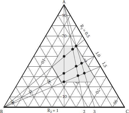
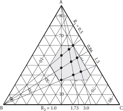
Figure 11.2 displays the individual constraints and ratios of components for the gasoline-blending example.

Before we discuss the design space, let’s first see how to draw in the ratio lines. With simple ratios such as these, it’s very easy. For R₁ (C/A), go to the C–A side of the triangle. The ratio of 1 is achieved at the midpoint, or 50/50 level. From there, draw a line to the opposite vertex (B). Along that line, the ratio of one for C/A is preserved. Similarly, you can establish an R₁ (C/A) ratio of 0.5 by choosing one-third (33.3%) of component C versus two-thirds (~66.7%) of A on the same (C/A) side of the trilinear graph. Again, draw a line to the opposite vertex (B). Finally, follow the same process to create a ray for an R₁ of 1.5. Next, we move on to R₂ (C/B). These ratios can be most easily established along the C–B side of the triangle. The ratio of 1 is at the 50/50 midpoint. That’s easy! Again, you can draw a line to the opposite vertex (A) from this point and thus preserve this ratio of 1. By the same procedure, we created rays for R₂ of 2 and 3.

Figure 11.2  Nine gasoline blends for 3² RSM design.

Now comes the fun part: the intersection of the three R₁ rays and the other three rays for R₂ ratios form the design. Notice that the resulting points provide a decent, but not an outstanding, coverage of the feasible mixture space. For example, it does not reach out to the corners, called extreme vertices. Nor does it center the middle points. As we warned you earlier, these less-than satisfactory design layouts are a drawback to the use of ratios, which becomes more pronounced as constraints become more complex. We will offer a better alternative after carrying this example along a bit further. There’s still much work to be done for executing and ultimately analyzing this experiment conducted in terms of ratios.

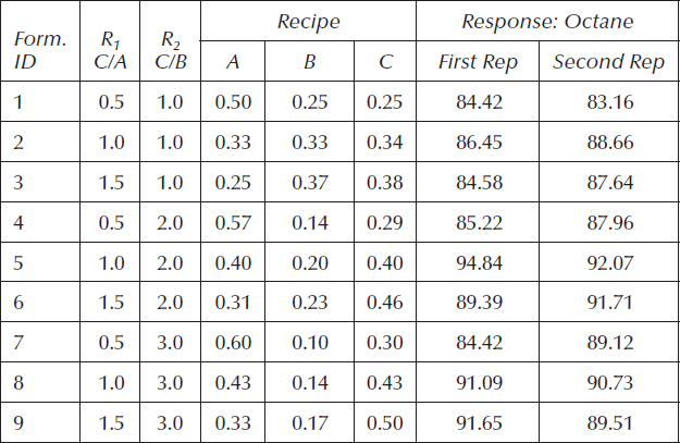
Table 11.2 shows the full three-level design in terms of ratios (R₁ and R₂), the back-calculated recipes (see the sidebar titled “The Tedious Downside of Formulating via Ratios” for details) for the three gasoline components (A, B, and C), and the measured response—the octane number of the resulting fuel. The design is fully replicated in a randomized manner, but for the sake of space, the two results at every unique formulation are tabulated side by side.

Table 11.2  Gasoline-Blending Experiment

THE TEDIOUS DOWNSIDE OF FORMULATING VIA RATIOS: CALCULATING RECIPES

It can be quite a chore to make the necessary translation of ratios, used to design an RSM experiment for formulation, back to the actual composition for use as a recipe sheet by the people doing the actual mixing. In the three-ingredient case for gasoline blending, we have three equations to work with—two for the ratios plus another for the overall constraint on the fixed total (100% or 1 on a scale of zero to one):

1.  R₁ = C/A

2.  R₂ = C/B

3.  A + B + C = 1

Then, with three equations for three unknowns, it’s simply (?) a matter of arithmetic^* to solve for the three components:

  A = R₂/(R₁ + R₁R₂ + R₂)

  B = R₁/(R₁ + R₁R₂ + R₂)

  C = R₁R₂/(R₁ + R₁R₂ + R₂)

*  Suggestion: Make use of readily available software that solves equations like these. Then, whether you calculate by hand or by a computer, check the recipes via a spreadsheet software package to ensure that each formulation adds up to the proper total and produces the specified ratios. This might save much time, trouble, and embarrassment.)

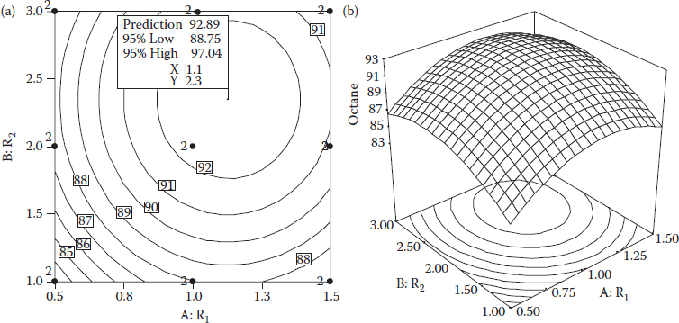
Via least-squares regression, the octane data were fitted to a quadratic polynomial equation to produce this predictive model:

${\displaystyle \widehat{\text{y}}}=92.36+1.68\text{A}+1.80\text{B}-3.24{\text{A}}^2-2.58{\text{B}}^2$

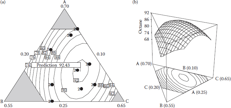
The 2FI (AB) was insignificant (p > 0.1), so it’s been removed. All other terms are significant at p ≤ 0.05. The LOF is insignificant (p > 0.1) and diagnostics on residuals appear to be normal; so, the model is deemed to be valid for predictive purposes (${\text{R}}_{\text{Pred}}^2=0.59$). Also, the adequate precision statistic of 10.2 far exceeds the guideline of 4; so, by this measure of signal to noise, the model scores very well. The contour plot (with the optimum flagged) and 3D response surface are displayed in Figure 11.3a and b, respectively.

Figure 11.3  (a) Contour plot for the gasoline case. (b) 3D surface for octane.

The optimum point (R₁ = 1.13 and R₂ = 2.35) translates (via the equations provided in the sidebar) to a composition of (0.38, 0.19, and 0.43) for (A, B, and C). It produces an octane of 93.

DEALING WITH NONLINEAR BEHAVIOR OF RATIOS

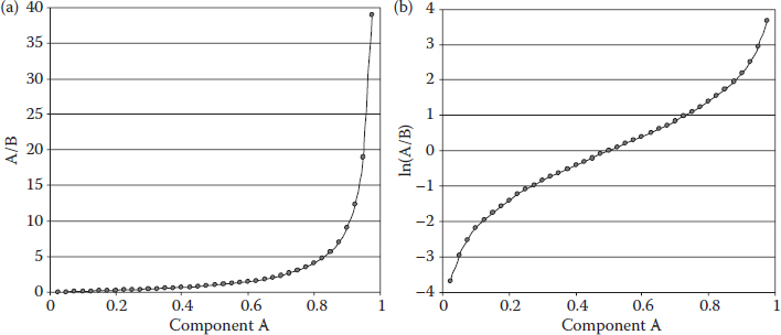
As you’ve seen in the gasoline-blending case, ratios do not provide a uniform coverage of the mixture space. In Figure 11.4a, you see a graph showing the ratio of A to B versus the level of A. Notice how it blows up as component A goes to a value of 1, because this drives B to 0, causing the ratio to become infinite. This can be counteracted to some extent by transformation with the logarithm (natural or base 10, it will not matter). Figure 11.4b displays a noticeably more linear response of ln(A/B) to A, particularly in the range from 0.2 to 0.8.

Therefore, we suggest that you consider averaging logarithms of the extreme ratios to determine the intermediate ratios. For example, in the gasoline-blending case, the middle values of the two ratios could be transformed as follows:

$\begin{array}{cc}{\text{R}}_1={\text{e}}^{\left((\ln (0.5)+\ln (1.5)/2)\right)}=0.866& {\text{R}}_2={\text{e}}^{\left((\ln (1.0)+\ln (3.0)/2)\right)}=1.73\end{array}$

Figure 11.4  (a) Ratio of two ingredients. (b) Ratio after being logged.

Figure 11.5  Layout of a gasoline-blending design with new midpoints based on log.

You can see how this improves the spacing of the middle points in Figure 11.5.

A Different Approach for Optimizing Formulations: Mixture Design

The use of ratios accounts for natural relationships in formulation components, such as the stoichiometry of a reagent to a catalyst in a chemical reaction. However, the predictive models in these terms cannot be interpreted very readily. It would be much handier to see the equation as a function of the original ingredients. This can be done via a polynomial form called Scheffé after the originator (Henri Scheffé, 1958). Here’s the predictive model for gasoline octane refitted to the Scheffé polynomial for mixtures:

${\displaystyle \widehat{\text{y}}}=75.80\text{A}+56.23\text{B}+73.77\text{C}+39.82\text{AB}+63.88\text{AC}+95.30\text{BC}$

Notice that all three components are detailed in this second-order (nonlinear) equation. Observe that all the coefficients for the interaction terms are positive. This indicates synergism between components—that is, more octane emerges from any two materials than can be expected from a simplistic linear-blending model of the two. In other words, two plus two equals more than four! Formulators are overjoyed when they see synergism like this, the most dramatic of which occurs between components B and C, as evidenced by their model coefficient being the largest of the second-order terms. This is graphically illustrated by the pronounced upward curve in the B–C edge of the 3D response surface graph shown in Figure 11.6b. (The hexagonal region covered is identical to that depicted earlier, except that it’s been magnified as far as possible within the boundaries of the trilinear graph.)

Now is a good time to return to the predictive model and observe from inspection of the coefficients for the main effects that material B falls short of the other two. Thus, on the 3D graph in Figure 11.6b, the response dives down toward the B corner of the trilinear mixture space. However, be careful to put too much stock in the linear coefficients when you constrain the ingredients. For example, in this case, the predicted value of 56.23 (the coefficient for B in the equation) is an extrapolation for the octane of the purest B—which, as you can see from the contour plot in Figure 11.6a, reaches a theoretical value of 0.55, but in actuality, B never exceeded 0.4 in the blending experiment. Remember the mantra of DOE: Never extrapolate!

Figure 11.6  (a) Trilinear contour plot for the gasoline case. (b) 3D surface for octane.

The optimum blend for octane is flagged on the contour plot in Figure 11.6a. It comes out to nearly the same composition (A = 0.4, B = 0.19, and C = 0.41) when predicted from the mixture model as it did from the original layout in ratio space. Whichever point of view is taken, the peak falls well within the explored space. However, as we’ve discussed, it’s obvious from the plotted design points that the experiment laid out via ratios did a poor job exploring the extreme compositions that were considered feasible for blending.

DERIVATION OF SECOND-ORDER SCHEFFÉ POLYNOMIAL

Here is the derivation of the second-order Scheffé polynomials for two components. It takes the inherent constraint of mixtures, that is, x₁ + x₂ = 1, into account.

$\begin{array}{l}{\displaystyle \widehat{\text{y}}}={\text{β}}_0+{\text{β}}_1{\text{x}}_1+{\text{β}}_2{\text{x}}_2+{\text{β}}_{12}{\text{x}}_1{\text{x}}_2+{\text{β}}_{11}{\text{x}}_1^2+{\text{β}}_{22}{\text{x}}_2^2\hfill \\ {\text{Replace β}}_0\text{by}{\text{β}}_0({\text{x}}_1+{\text{x}}_2);{\text{x}}_1^2\text{by}{\text{x}}_1(1-{\text{x}}_2);{\text{x}}_2^2\text{by}{\text{x}}_2(1-{\text{x}}_1):\hfill \\ {\displaystyle \widehat{\text{y}}}={\text{β}}_0({\text{x}}_1+{\text{x}}_2)+{\text{β}}_1{\text{x}}_1+{\text{β}}_2{\text{x}}_2+{\text{β}}_{12}{\text{x}}_1{\text{x}}_2+{\text{β}}_{11}({\text{x}}_1(1-{\text{x}}_2))+{\text{β}}_{22}({\text{x}}_2(1-{\text{x}}_1))\hfill \\ {\displaystyle \widehat{\text{y}}}=({\text{β}}_0+{\text{β}}_1+{\text{β}}_{11}){\text{x}}_1+({\text{β}}_0+{\text{β}}_2+{\text{β}}_{22}){\text{x}}_2+({\text{β}}_{12}-{\text{β}}_{11}-{\text{β}}_{22}){\text{x}}_1{\text{x}}_2\hfill \\ {\displaystyle \widehat{\text{y}}}={\text{β}}_1^{\prime }{\text{x}}_{\text{1}}+{\text{β}}_2^{\prime }{\text{x}}_{\text{2}}+{\text{β}}_{12}^{\prime }{\text{x}}_{\text{1}}{\text{x}}_{\text{2}}\hfill \\ \text{where}{\text{β}}_1^{\prime }={\text{β}}_0+{\text{β}}_1+{\text{β}}_{11},{\text{β}}_2^{\prime }={\text{β}}_0+{\text{β}}_2+{\text{β}}_{22}\text{and}{\text{β}}_{12}^{\prime }={\text{β}}_{11}-{\text{β}}_{22}\hfill \end{array}$

These models, geared to mixtures, are distinguished by their lack of intercept. (The Scheffé coefficients incorporate the intercept [β₀] from the original equation.) What is the meaning of an intercept in mixtures? It would be the response when all the components are 0—this can’t exist!

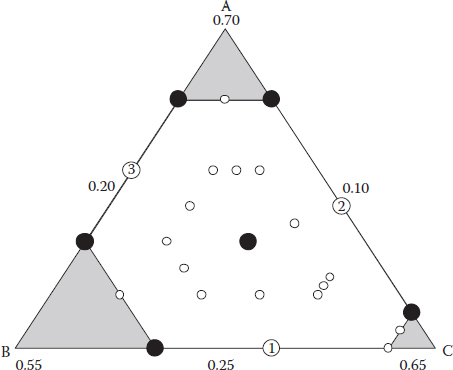
The gasoline-blending case presents an ideal application for an optimal design along the lines discussed in Chapter 7, where we introduced complex constraints as an aspect of RSM. Aided by Design-Expert software, we laid out the optimal mixture design shown in Figure 11.7. It’s geared to fit a quadratic Scheffé polynomial. We then augmented the base optimal design (the six black circles) with three additional unique blends (open circles numbered in order of being picked) to test for LOF and match up with the original case that features nine compositions. This latter set of runs, called “check blends,” is picked via the distance-based criterion. The remaining blank circles show candidate points that did not get chosen by either the optimal or the distance-based augmentation.

All nine of the chosen points could be replicated for the estimation of pure error, the same as before. At the very least, we’d recommend that the four most extreme vertices be replicated at random intervals in the blending runs. Another good candidate for replication would be the point in the middle—called the centroid in the jargon of the mixture design.

We’ve only scratched the surface of the mixture design. For more detail, see the two referenced texts by Cornell (2002) and Smith (2005). As you will see in Problem 11.2, setting up formulation problems via the tools of the mixture design is much more straightforward than taking the ratio route. These designs, being tailored to the mixture space, include more extreme compositions, that is, they are space filling, thus generating bigger effects that are more likely to emerge as significant signals. The use of Scheffé polynomials, the standard model for the mixture design, facilitates the interpretation of the component effects and interactions. If you get involved in formulation work, we urge you to look into this powerful tool for RSM.

Figure 11.7  An alternative RSM design based on an optimal criterion for mixture space.

PRACTICE PROBLEMS

11.1  You will be glad that we left this problem for last because it’s a lollapalooza! A flexible part manufactured for medical use is made from four primary components:

  Resin A

  Crosslinker B

  Polymer X

  Polymer Y

The recipe for making this part is laid out as follows with the acceptable ranges listed:

1.  Resin: 35–50 wt.% of copolymers (X and Y)

2.  Crosslinker: 10–15 wt.% of copolymers

3.  Polymer ratio: 60/40–80/20 X to Y

The response is elongation—the higher the better. A BBD will be done to optimize the formulation on the basis of this response. But first, some work must be done to set up proper ratios and translate them back to an actual composition.

The ratios can be defined as follows:

  R₁ = A/(X + Y)

  R₂ = B/(X + Y)

  R₃ = X/Y

Table 11.3 shows the ranges of the ratios to be studied via the BBD. For reasons described in the sidebar titled “Dealing with Nonlinear Behavior of Ratios,” it will be laid out in terms of natural logarithms (shown in parentheses).

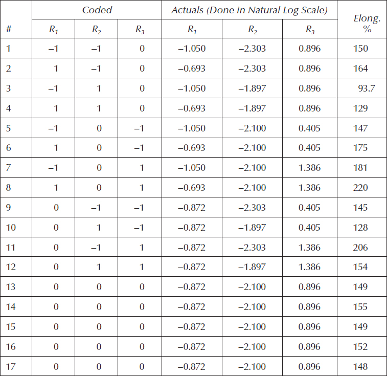
The resulting BBD is shown in Table 11.4. We translated back from the log scale to the original ratios by taking antilogs. These will then be converted into compositions for experimental purposes. However, given the responses for elongation listed in Table 11.4, along with the layout of inputs in log scale, you can develop a predictive model and perform the optimization (maximize).

Table 11.3  Ratio Constraints

Ratio	Description	Ratio Range	Low – (ln)	High + (ln)
R1	Resin A as percent of the copolymer	35%–50%	0.35 (−1.050)	0.5 (−0.693)
R2	Crosslinker B as percent of the copolymer	10%–15%	0.10 (−2.303)	0.15 (−1.897)
R3	Polymer X to polymer Y	60/40–80/20	1.5 (0.405)	4.0 (1.386)

The mixture constraint is

  A + B + X + Y = 1

From this and the ratio equations, the actual composition of the polymer is derived as follows:

  A = R₁/(R₁ + R₂ + 1)

  B = R₂/(R₁ + R₂ + 1)

  X = R₃/(R₃ + 1)(R₁ + R₂ + 1)

  Y = 1/(R₃ + 1)(R₁ + R₂ + 1)

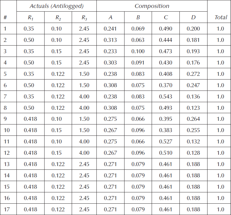
Table 11.5 shows the compositions based on the ratios from Table 11.4 for the BBD. This is necessary for carrying out the experiment.

Ultimately you must translate the optimum point predicted from your model back to a composition by going through the same process detailed in Table 11.5:

1.  Antilog each of the factor levels to translate them into actual ratios

2.  Plug and chug these through the ratio equations to solve for A, B, X, and Y, the resin, crosslinker, and two polymers, respectively.

We never said this problem would be easy!

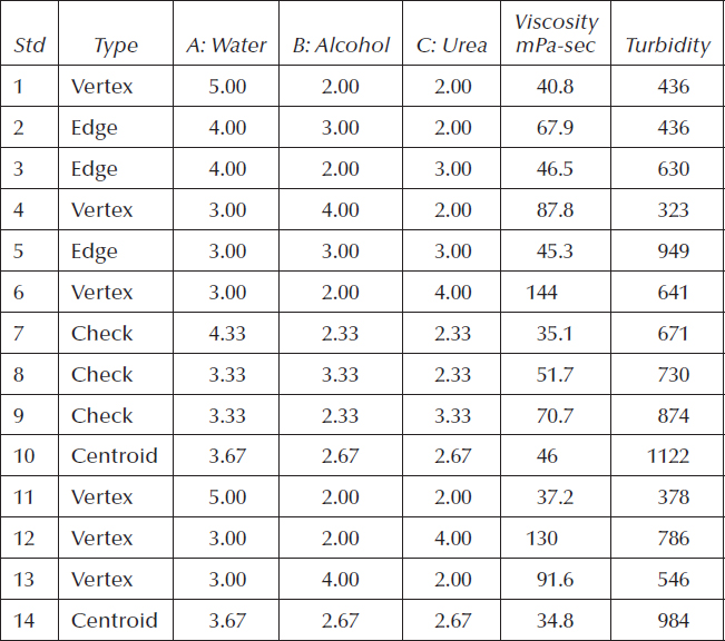
11.2  If you are not up to going through all the gyrations of applying RSM to formulations via the use of ratios, consider doing it in a more straightforward manner via the mixture design. From the website for the program associated with this book, follow the “Mixture Designs” link to a tutorial that provides an introduction to statistical tools for formulation developers. It details a case study on a detergent for which two responses were deemed to be the most important:

1.  Viscosity

2.  Turbidity

Table 11.4  BBD on Formulation for Medical Part

The formulators varied three components as shown below

  3% ≤ A (water) ≤ 8%

  2% ≤ B (alcohol) ≤ 4%

  2% ≤ C (urea) ≤ 4%

They required that these three active components always equal 9 wt.% of the total formulation, that is,

$\text{A}+\text{B}+\text{C}=9\%$

The other components (held constant) then must equal 91 wt.% of the detergent. Table 11.6 shows the experimental recipe sheet.

Table 11.5  Compositions for Experiment on Medical Part

Note that the last four runs in standard (Std) order are replicates of the three vertices in the triangular mixture space (a simplex) and the overall centroid (the equivalent of a CP in an RSM design). You will see the design pictured in the software tutorial (and perhaps on screen as well, if you bring up the program on your computer). We dare not get into any more detail—that must await another book devoted to simplifying the mixture design. The first several chapters have been written and posted as a primer posted at www.statease.com/formulator. Check it out!

Table 11.6  Mixture Design for a Detergent