6   STYLE

All art is collaboration, and there is little doubt that in the happy ages of literature, striking and beautiful phrases were as ready to the story-teller's hand as the rich cloaks and dresses of his time.

—J. M. Synge, preface to Playboy of the Western World

In statistical or quantitative authorship attribution, a researcher attempts to classify a work of unknown or disputed authorship in order to assign it to a known author based on a training set of works of known authorship. Unlike more general document classification, in authorship attribution we do not want to classify documents based on shared or similar document content. Instead, the researcher performs classification based upon an author's unique signal, or “style.” The working assumption of all such investigation is that writers have distinct and detectable stylistic habits, or “tics.” A consistent problem for authorship researchers, however, is the possibility that other external factors (for example, linguistic register, genre, nationality, gender, ethnicity, and so on) may influence or even overpower the latent authorial signal. Accounting for the influence of external factors on authorial style is an important task for authorship researchers, but the study of influence is also a concern to literary scholars who wish to understand the creative impulse and the degree to which authors are the products of their times and environments. After all, in the quarry of great literature, it is style, or “technique,” that ultimately separates the ore from the tailings.* To greater and lesser extents, individual authors agonize over their craft. After a day spent working on two sentences of Ulysses, James Joyce is reported to have said in response to a question from Frank Budgen: “I have the words already. What I am seeking is the perfect order of words in the sentence” (Budgen 1934, 20).† Some readers will prefer Stephanie Meyer to Anne Rice or Bram Stoker, but when the plots, themes, and genre are essentially similar, reader preference is, in the end, largely a matter of style.

No computation is necessary for readers to distinguish between the writings of Jane Austen and Herman Melville; they write about different subjects, and they each have distinct styles of expression. An obvious point of comparison can be found in the two writers’ use of personal pronouns. As a simple example, consider how Austen, who writes more widely about women than Melville, is far more likely to use feminine pronouns. In Sense and Sensibility, for example, Austen uses the female pronoun she 136 times per 10,000 words. In Moby Dick, Melville uses she only 5 times per 10,000.* This is a huge difference but one that is not immediately obvious, or conscious, to readers of the two books. What is obvious is that there are not many women in Moby Dick. Readers are much more likely to notice the absence of women in the book than they are to notice the absence of feminine pronouns; even the most careful close reader is unlikely to pay much attention to the frequency of common pronouns.† It is exactly these subtle “features” (pronouns, articles, conjunctions, and the like), however, that authorship and stylometry researchers have discovered to be the most telling when it comes to revealing an author's individual style.‡ There are, of course, other stylistic differences that are quite obvious, things that leap out to readers. These are not primarily differences in subject matter but differences in the manner of expression, in the way authors tell their stories. One writer may use an inordinate number of sentence fragments; another may have a fondness for the dash. When these kinds of obvious difference are abundant, and when we simply wish to identify their presence in one author, the use of computation may be unnecessary. Joyce has the habit of introducing dialogue with a dash, whereas D. H. Lawrence does not. The differences between these two writers with regard to the dash are rather striking. Often, however, the differences are not so striking: attributing an unsigned manuscript to one or the other of the Brontë sisters would be a far more challenging problem; their linguistic signatures are quite similar to each other.

For the sake of illustration, let's imagine a researcher has discovered an anonymous, unpublished manuscript. External evidence shows that either Melville or Austen wrote it. For simplicity, assume that Melville and Austen published only the two aforementioned books, Sense and Sensibility and Moby Dick. After calculating the relative frequency of she in the anonymous text at 86 occurrences per 10,000 words, we might be fairly confident in asserting that Austen, with an average of 94, is the likely author—Melville, remember, uses she just 4–5 times per 10,000. However unlikely, it remains possible that the unknown text is in fact a story by Melville with a female protagonist and thus has many more feminine pronouns than what one finds in Moby Dick. Were authorship-attribution problems as simple as comparing the use of a single feature, then they would not be problems at all!

Real problems in computational authorship attribution are far more complicated and subtle than the above, one-feature, example. In fact, these problems involve processing “high-dimensional” data. To explain this concept requires expansion of our current example to include a second word; we add the male pronoun he. When it comes to Sense and Sensibility and Moby Dick, the results are almost identical: 63 occurrences per 10,000 for Sense and Sensibility and 64 for Moby Dick. Plotting these pronoun measurements on a two-dimensional grid, in which the y axis is the measure of he and the x axis the measure of she, results in the two-dimensional graph seen in figure 6.1. On the y axis, both authors are close to each other, but they are quite far apart on the she x axis. Were we to calculate the relative frequency of he for the anonymous text at 54 occurrences per 10,000 and plot it alongside Melville and Austen, we would see that in terms of these two dimensions, the anonymous text is much “closer” to Austen, where she occurred 86 times per 10,000 words (figure 6.2). Still, this would not be very convincing evidence in support of an attribution to Austen. To be convincing, the researcher must account for many more features, and since the number of dimensions corresponds to the number of features examined, any charting of distances quickly goes beyond what can be represented on a two-dimensional x-y grid. Imagine adding a third word feature, the word it, for example. By extending a z axis back in space, the relative frequencies of it in Melville, Austen, and the anonymous text could be plotted, as in figure 6.3. The task would now be to identify which author is closest to the anonymous text in a three-dimensional space. Add a fourth or fifth feature, and things get complicated. Whereas the human mind is incapable of visualizing this problem much further than three dimensions, mathematics is not so hobbled, and there are a variety of statistical methods for plotting and calculating distances between objects in multidimensional space.

Principal component analysis was one of the earliest statistical techniques applied to this multidimensional problem (see, for example, Burrows 1989). PCA is a method of condensing multiple features into “principal components,” components that represent, somewhat closely, but not perfectly, the amount of variance in the data.* More recently, authorship researchers have adopted statistical methods from the machine-learning literature.† Generally speaking, these methods involve some form of supervised classification: a process that involves “training” a machine to recognize a particular author's feature-usage patterns and then allowing the machine to classify a new text according to how well it “matches” or is similar to the training data. Unlike PCA, these methods are designed to grapple with all of the features in a high-dimensional space. As such, these classification results are often more interpretable.‡ Whereas PCA condenses features into components, these techniques keep the features as distinct dimensions.

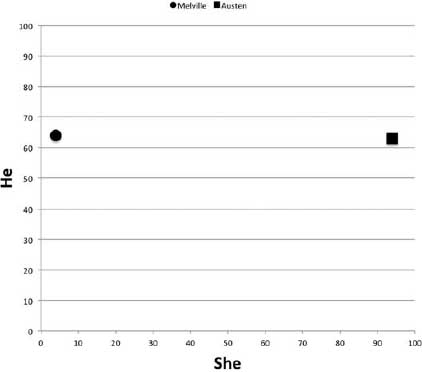
Figure 6.1. Two-dimensional feature plot with two books

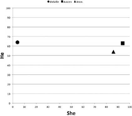
Figure 6.2. Two-dimensional feature plot with three books

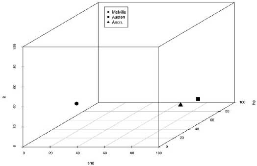
Figure 6.3. Three-dimensional feature plot with three books

Even with a suitable statistical method and an appropriate feature set, there are still outstanding problems that challenge authorship-attribution researchers. In particular, there is the challenge associated with not knowing exactly what is responsible for the usage patterns measured in the feature set. For example, if the training samples include nonfiction texts and the text to be identified is fictional, it may be that the different usage patterns detected are better attributed to genre differences than to authorial differences. In an ideal authorship case, the training data and the test data are as homogenous as possible. The Federalist Papers, studied extensively by Mosteller and Wallace (1964) in their landmark work, serves as an ideal case. Of the eighty-five Federalist Papers, fifteen are considered to be of unclear authorship. But each of the fifteen disputed papers is known to have been written by at least one of three men: James Madison, Alexander Hamilton, and John Jay.* The undisputed papers offer an ample collection of works by Madison, Hamilton, and Jay for use in training a classifier. Because all the papers deal with the same subject and are of fairly uniform length, the Federalist Papers is considered by many to be an ideal corpus for authorship-attribution research, and, as R. S. Forsyth noted some years ago, the Federalist Papers problem “is possibly the best candidate for an accepted benchmark in stylometry” (1997). But researchers rarely find such well-defined and well-controlled problems. They must inevitably grapple with the possibility of unknown external factors influencing their attribution results and offer caveats when it comes to the role that nonauthorial factors such as genre may or may not play in the determination of style. Because each problem is unique, there is no simple way of defining or accounting for the extent to which factors external to an author's personal style may influence a given composition.

In recent work analyzing the degree to which novelistic genres express a distinguishable stylistic signal, my colleagues and I were faced with a problem of having to assess how much of a detected “genre” signal could be reasonably attributed to the conventions of the genre and how much of the signal was likely to be attributable to other factors, such as author, time period, or author gender. The work began as a collaboration with Mike Witmore of the University of Wisconsin. Witmore and his colleague Jonathan Hope had published a series of papers that used a software package called Docuscope to extract features from Shakespeare's plays. These features are called Language Action Types, or LATs (Hope 2004; Witmore 2007). Using these LATs, Witmore and Hope machine-clustered Shakespeare's plays into categories that aligned extremely well with our human-defined genre classes of “history,” “tragedy,” and “comedy.” After learning of Witmore's results, Franco Moretti was interested to see whether the same technique could be employed to classify nineteenth-century novels into their novelistic subgenres (for example, “Bildungsroman,” “national tale,” “Gothic,” and so on). If the techniques were successful, then there would be evidence to support the hypothesis that genre operates at a lexical, linguistic, and stylistic level. Through analysis of the features used in the clustering, a variety of assertions about how the different genres are “expressed” might be made. The research team at the Stanford Literary Lab compiled a corpus of 106 nineteenth-century novels, and Moretti identified each according to novelistic genre. Each novel was then segmented into tenths, for a total of 1,060 segments. Witmore was given these data without any identifying information—title pages were stripped out—and his task was to work over the data with his methods and then report his findings at Stanford in February 2009. The results of Witmore's experiment were impressive, and the entire experiment was later documented in “Quantitative Formalism: An Experiment,” published in Pamphlet One of the Stanford Literary Lab (Allison et al. 2012).

At the same time that Witmore was preparing his results, I began a series of parallel experiments. Witmore's work used Docuscope to convert lexical information into LATs, which were then counted, normalized, and used as features in his clustering procedures. For the parallel experiments, frequently occurring words and punctuation tokens were extracted and used as the basis for a feature set. Any word or mark of punctuation with a mean relative frequency across the corpus of above 0.03 percent was selected.* This resulted in a feature set of 42 high-frequency word and punctuation types: a matrix of 1,060 texts by 42 features with measurements of relative frequency for each.† Using these features, an unsupervised clustering of the data was performed: first a distance matrix computation was applied and then a hierarchical clustering analysis.‡ The procedure calculates the Euclidian distance between the texts and then groups them according to the “closeness” of their individual signals. The results were startling: using just 42 features, the routine not only grouped chunks from the same texts together (an unsurprising result in itself), but also grouped works from the same genres in close proximity. The results suggested that there were grounds for believing that genres have a distinct linguistic signal; at the same time, however, a close analysis of the data tended to confirm the general consensus among authorship-attribution researchers, namely, that the individual usage of high-frequency words and punctuation serves as an excellent discriminator between authors. In other words, though genre signals were observed, there was also the presence of author signals and no obvious way of determining which feature-usage patterns were most clearly “authorial” and which “generic.”

Although the results were encouraging, they forced us to more carefully consider our claims about genre. If genres, like authors, appear to have distinguishable linguistic expressions that can be detected at the level of common function words, then a way was needed for disambiguating the “author” effects from those of genre and for determining whether such effects were diluting or otherwise obscuring the genre signals we observed. If there were author effects as well as genre effects, then one must consider the further possibility that there are generational effects (that is, time-based factors) in the usage of language: perhaps the genre signals being observed were in fact just characteristic of a particular generation's habits of style. In other words, although it was clear that the novels were clustering together in genre groups, it was not clear that these groupings could be attributed to signals expressed by unique genres. Although the results looked compelling, they were not satisfying. A way of separating and controlling for author, gender, and generation was required.

In the initial experiment, unsupervised machine clustering was used to “sift” the texts based on similarities in common-word and punctuation usage. In machine clustering, the objective is to group similar items into clusters. We get an algorithm and feed it a lot of information about our novels and ask it to group the novels into clusters based on how similar they are to each other. We measure similarity in this case based on a set of variables or features. If we were clustering shapes, for example, we might have a feature called “number of sides.” The computer would cluster three-sided objects into one pile and four-sided objects into another; the machine would not know in advance that these shapes were examples of what we call “triangles” and “squares.” In machine clustering, an algorithm assesses all the data at once with no prior information about potential groupings. The process clusters novels with similar data patterns together, and these data can be plotted in a treelike structure that links the genres based on similarity across the 42 features (figure 6.4). It is up to the researcher to then assess the outcome and determine the extent to which the clusters make human sense. The clusters of genres in figure 6.4 do make sense. Industrial novels grouped together, as did the Bildungsroman novels. Gothics clustered with historical novels and so on. The results conform to our human expectations, which are, of course, based on our human “definitions” of what constitutes these genres in the first place.

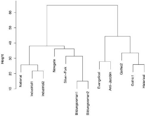
Figure 6.4. Cluster dendrogram of genres

In a supervised experiment, however, the goal is not to cluster similar objects, but to classify an unknown text, or texts, into any one of a set of predefined categories or classes. The researcher groups and labels a set of “training texts” in advance, and the machine uses this information to build a “model.” The machine assesses a new text and places it into the most similar of the previously defined categories that the model has learned. Once the model is constructed, a new text can be analyzed and “classified” into one of the existing categories. This is an approach frequently used in authorship attribution: the process assigns an anonymous text to a known author within a closed set of candidates. In the case of this genre experiment, however, there are no texts of unknown origin; we already know “the answers.” Instead of trying to classify some unseen text into a known category, the goal here is to use the machine to assess the relative strength of the genre signal against the other potential signals. Because we already know the “correct” answers, the accuracy of the classification can be known with absolute certainty, and the accuracies can then be compared across different tests. In other words, it is possible to apply the techniques of authorship attribution as a way to investigate factors other than author.

To investigate this matter thoroughly, a process of iterative sampling is required. Using scripts written in R, an iterative experiment was conducted in which with each iteration two-thirds of the texts in the data set were selected at random for training a model, and the remaining one-third were held out as “test” data for classification. After each iteration of sampling and classification, the rate of classification error was recorded. The rates of error were then averaged over the number of runs of the process to arrive at an average or expected rate of error. When conducting this experiment using novelistic genre as the predefined class, an error rate of 33 percent was observed.* In other words, given this closed set of 1,060 text segments from 106 nineteenth-century novels, the algorithm could correctly guess the segment's genre 67 percent of the time. Considering the fairly high number of available classes (twelve genres) and the relatively small number of samples, 67 percent was a decent average.† Nevertheless, this figure, which represents the mean number of cases in which a correct result was returned, tells only part of the story. To fully understand the results requires analysis of the resulting confusion matrix, which measures the “precision” and “recall” of the classification.

Precision is a measurement of the number of “true positives” for any given class divided by the sum of the true positives and false positives. In other words, we divide the number of times that the machine correctly guessed “Gothic” by how many times it guessed “Gothic” overall (including the incorrect guesses). Precision is, therefore, a measure of correct Gothic guesses (true positives) versus incorrect Gothic guesses (false positives).‡ Recall, on the other hand, is a measurement of the number of true positives divided by the actual number of items in the class; or, to put it another way, recall is the number of correctly guessed Gothic texts divided by the sum of correctly guessed Gothic texts and texts that should have been identified as Gothic but were classified as something else. Table 6.1 shows the full confusion matrix for the genre test.

In this experiment, the classifier achieved the highest degree of precision (88 percent) when classifying the sensation novels. Of the thirty-four sensation (“Sens”) assignments, only four were incorrect. For sensation novels, recall was also fairly good, at 75 percent. The classifier correctly identified “Sens” in 75 percent of the novel fragments that were in fact sensation novels. National (“Natl”) novels present a different case. Precision for national novels was just 48 percent, meaning that only 48 percent of the “national” guesses that the classifier made were in fact true positives. In other words, the national “genre signal” that the machine established during training was relatively weak and was frequently “misdetected” in novels of other genres. Recall, however, was exceptional, meaning that when the actual genre class was national, the classifier rarely misclassified it as something else. This does not necessarily mean that the national model was especially good at classifying national novels; it could mean that the signals the model constructed for the other genres were comparatively better, and the national signal became a kind of default assignment when none of the other genre signals offered a strong match.

In fact, every assignment that the model makes is based on a probability of one class versus another, and in some cases the most probable choice is only slightly better than the second most probable choice. Take the case of a randomly selected text sample from the data: a sample with the unique ID 642. This text sample is from an anti-Jacobin novel, and the classifier correctly classified it as anti-Jacobin with 99.3 percent probability over the other genre classes in this closed set of genres. The next closest genre assignment was evangelical with 0.04 percent. In this case, the classifier is very confident about its selection of anti-Jacobin. Less certain is the machine's classification of sample ID 990, which is a segment from a Gothic novel. The machine misclassified sample 990 as anti-Jacobin with 52 percent probability. The second-place candidate, however, was Gothic, the correct genre, to which the machine assigned a probability of 47 percent. The choice the machine made between Gothic and anti-Jacobin for this particular segment was based on a very small probability margin. Were we not dealing with a computer and statistics, one might even say that the choice was “not an easy one to make.” Text sample 990 had much about it that seemed anti-Jacobin and much about it that seemed Gothic. Given the reality of these “close-call” situations, it is useful to consider both the first- and the second-place assignments when assessing the overall performance and value of the model, especially so when we consider that the classes that we are dealing with here, genres, are human inventions that are not always clearly delineated and can “bleed” into each other. We might, for example, find a novel that is in our human estimation composed of equal parts Bildungsroman and silver-fork.*

Table 6.1. Twelve novelistic subgenres

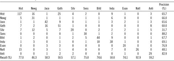
Note: The categories are as follows: historical, Newgate, Jacobin, Gothic, silver-fork, sensation, Bildungsroman, industrial, evangelical, national, and anti-Jacobin.

If we consider either a first- or a second-place assignment as an “accurate” or useful assignment, then overall model quality looks quite a lot better. Figure 6.5 shows the percentage of correct assignments for each genre when “accuracy” is defined as a true positive in either the first or the second place. The genres in figure 6.5 are sorted from left to right based on the accuracy of the first, or primary, assignment. So, while sensation and industrial novels have the highest percentage of correct first-place assignments, 100 percent of Newgate and evangelical novels are assigned as either first or second most probable.

In order to contextualize these data, it is instructive to examine the places where the classifier went wrong, the misclassifications. When a novel segment is assigned to the wrong class, it is useful to know what that wrong class is. It is particularly useful to know if a specific type of incorrect class assignment occurs frequently. For example, when Bildungsroman segments are misclassified, they are most often (50 percent of all the misclassifications) classified as industrial novels, a fact that suggests that there may be some linguistic or stylistic affinity between the Bildungsroman and industrial novels in these test data. Figure 6.6 shows a breakdown of the misclassified Bildungsroman novel segments.

An examination of figure 6.5 and figure 6.6 provides us with a way of better understanding not only the stylistic signal of genres but also the extent to which genres share stylistic affinity. For example, every one of the Bildungsroman novels that was misclassified in first place as industrial was correctly identified in the second-place position as Bildungsroman. In other words, there appears to be a special affinity between Bildungsroman and industrial novels when it comes to the usage of these high-frequency words and marks of punctuation. What exactly this stylistic affinity is requires a still deeper analysis of the data returned by the algorithm; however, it is interesting to note here that the Bildungsroman segments that were misclassified as industrial novels were also all from novels roughly within the time period that we typically associate with the industrial. The segments misidentified as industrial came from Thackeray's Pendennis (1849) and from two novels by George Eliot, Middlemarch (1872) and Daniel Deronda (1876). Given that Eliot's 1866 industrial novel Felix Holt is also in the data set, it is natural to wonder whether the misassignments here could be attributed to a latent author signal overpowering the forces of genre. Alternatively, it may be that the pull toward industrial is in fact a “generational” force. Is it perhaps not genre style at all but some other factor that is influencing these misclassifications? Before exploring this possibility, a few final observations are in order, so that we might fully understand the scope and diversity of evidence made available to us for analysis.

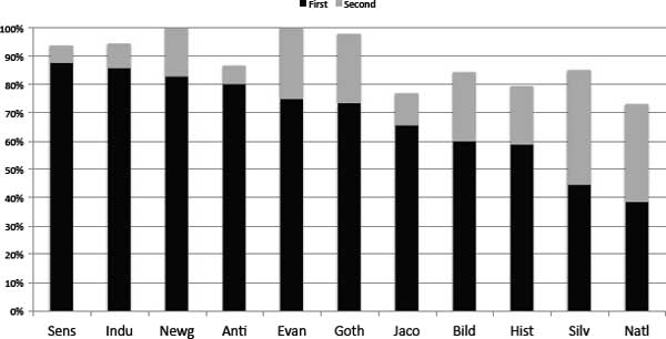
Figure 6.5. First-and second-place genre assignments

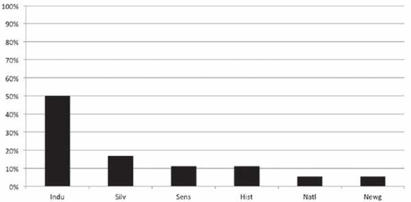
Figure 6.6. Incorrect assignment of Bildungsroman novels

• • •

In addition to the data already discussed, the machine also provides information about the features used in the analysis and which among these features proved most useful in separating between the different classes. For example, three features that are positively correlated with the Bildungsroman are the word features like, young, and little, which is to say that these three words are overrepresented in Bildungsroman novels compared to the other genres in the test data. Alternatively, the words upon, by, and this are underutilized in the Bildungsroman compared to other genres. The comma finds greatest expression in the national tale but is comparatively absent from sensation novels, where there is a preference for the period. Like the national tale, historical novels also overutilize the comma at the expense of the period. The exclamation mark appears prominently in Newgate novels, unsurprising given the nature of the genre, but is relatively absent from evangelical novels. This is by no means an exhaustive analysis of the available features or their relative weights within each class; such an analysis would amount to a discussion of 1,932 unique data points. Instead, these features represent a sampling of the richness of data available for interpretation. In other words, although it is clear that there is stylistic separation between the genres, it is not obvious why that separation exists or how that separation is embodied in the texts. The answer to the question of why undoubtedly lies in the details of the relative feature weights and requires careful analysis and interpretation in order to be able to move from the individual features toward a larger-scale description of how these features constitute a particular genre.

In prior work (Allison et al. 2012), my colleagues and I speculated that a high incidence of locative prepositions in the Gothic novel is a direct result of the genre's being heavily “place oriented.” As such, this genre demands a relatively greater frequency of locative prepositions in order to situate the novel's settings in space. This current investigation reveals strong evidence that there are even deeper subtleties of style, of linguistic usage, lurking beneath the surface of our long-established, noncomputational taxonomy of genre. Though not necessarily obvious or apparent to readers, these linguistic nuances are detectable by machine and lead us not only to a deeper understanding of the genres, which they define, but also to clearer definitions of genre itself.

Like the earlier experiments with clustering described in “Quantitative Formalism” (Allison et al. 2011), the supervised classification tests conducted here have added support to the hypothesis that genres indeed have a distinct stylistic signature, and they demonstrate that a genre signal exists and can be detected at the level of high-frequency word and punctuation features. The possible presence of other influential factors—factors such as time period, nationality, author, and author gender, for example—requires deeper investigation. Before we can argue that genres have measurable linguistic fingerprints, we must be able to isolate those feature fluctuations that are attributable only to genre and are not simply artifacts of some other external factor.

A further experiment was constructed using the same set of 106 novels but expanding the feature set from the 42 most frequent features to include all lexical and typographical elements exceeding a mean relative frequency threshold of 0.005. The idea was to expand the feature set in such a way that more features were included but context-sensitive features were still excluded. As noted previously, this feature winnowing, or “culling,” is designed to exclude context-sensitive words that might bias a classifier in favor of texts that share a common subject and not simply a similar style. A visual inspection of the word list suggested that .005 was an effective frequency threshold, one that selected few context-sensitive words.* Novel segmentation remained the same: each book was divided into 10 equal-size sample fragments. The result of this preprocessing and feature extraction was a data matrix of 1,060 segment “rows” by 161 feature “columns.” A unique ID further identified each sample, and to each row five additional metadata fields were added, indicating the gender of the author, the genre of the sample, the decade of publication, the author, and the title of the novel from which the sample was extracted.† The objective was to then analyze and rank each of the five metadata categories in terms of their effectiveness in accurately predicting the classes of the test data. Or, put another way, the goal was to assess which of these five categories “secretes” the strongest linguistic signal as measured by overall classification accuracy and by precision and recall. Complicating matters, however, each of the five categories has a different number of classes and thus presents a different degree of difficulty for the classifier. This in turn makes the simple comparison of accuracies problematic. With gender, for example, there are only two possible classes, male or female, whereas there are 47 different authors and 106 different titles in this data set. Thus, any comparison of relative strengths must take into consideration both the difficulty of the specific classification problem and the overall classification accuracy result. Ultimately, the relative strength of the five categories—calculated in terms of their predictive power—must be determined. Only then does it become possible to construct a hierarchy of signal strengths and thereby rank the stylistic pull associated with each category of metadata.

Unlike a real classification problem, in which there is some hitherto unclassified text of unknown origins, in this experiment all of the true classes are already known in advance. Because the classes are known in advance, the effectiveness of the classification process can be measured with perfect accuracy. Instead of using the classifier to guess the most likely source of a particular signal, the classifier's output is used as a way of gauging the signal strength of the sources. The classifier becomes a means for better understanding the interrelationships of the five categories with the linguistic data—the assumption being that the stronger the linguistic signal, the more accurate the classification accuracy. In other words, the classifier can be used to help understand which of the five different categories exerts the most influence on the resulting patterns found in the linguistic data. By way of analogy, we might imagine a clinical trial in which we wish to understand the factors influencing the effectiveness of a new blood-pressure drug. In this hypothetical trial, we begin by evaluating a patient's weight, age, gender, height, and beginning blood pressure. We then administer the drug. At the end of the trial, we measure the blood pressure and assess the degree to which the drug was effective. However, we also must look for any correlation between overall effectiveness and any one or more patient features that we evaluated at the beginning of the trial. For example, it may be discovered that the age of a patient influences the efficacy of the drug; for example, patients over fifty do not respond to treatment.*

To test the predictive power of each metadata category, the Nearest Shrunken Centroid (Tibshirani et al. 2003) classification algorithm was employed.† The NSC is a subtype of “nearest centroid” algorithms that begin by computing a standard centroid* for each class, calculating the average frequency for a feature in each class, and then dividing by the in-class standard deviation for that feature. The NSC takes an additional step of shrinking the centroids in a way that has the end result of eliminating features that contribute “noise” to the model.† Although the NSC was developed to aid in the diagnosis of cancer types through the analysis of gene-expression data, it has been shown to perform well in stylistic analysis, especially so in authorship attribution (Jockers, Witten, and Criddle 2008; Jockers and Witten 2010).‡ From a statistical perspective, the two types of problems (genetic and stylistic) are similar: both are composed of high-dimensional data, and the linguistic features are roughly analogous to the individual genes.

For each metadata category (gender, genre, decade, author, text), the model is run, and a tenfold cross-validation provides the resulting rates of error. These errors are averaged to generate an overall estimate of accuracy for each category.§ The average rates of error and accuracy are recorded in table 6.2. The cross-validation results indicated that “decade” was the weakest influence and “author” the strongest. However, as noted previously, each rate of error must be understood in the context of the number of potential classes within the category and in terms of both precision and recall. For example, “gender” involves classifying samples into one of two possible classes (male or female). A classifier guessing purely at random could be expected to guess correctly 50 percent of the time (at least in cases where there were equal numbers of male and female test samples).¶ Thus, with an overall error rate of 20 percent, the gender-based model is 1.6 times better than chance. Thought of another way, the addition of the linguistic data improves classification accuracy from 50 percent to 80 percent.# For “decade” there are ten potential classes, so a classifier guessing at random could be expected to guess correctly 10 percent of the time. In this experiment, we observe 53 percent correct classifications, 5.3 times better than chance. In the case of “genre” where there are twelve potential classes and an expected rate of accuracy of 8.3 percent, a classification accuracy rate of 67 percent was observed. This result is eight times better than chance. For “text” there were 106 potential classes. This is clearly the most challenging of the five problems. Based on chance alone, less than 1 percent (0.94) could be expected to be classed correctly. However, 85 percent of the classifications are correct for a result that is 90 times better than chance alone. Finally, for “author” there are 47 potential classes. We should expect 2.1 percent correct assignments by chance; nevertheless, 93 percent of the samples were classed correctly for a result that is 44 times better than chance! This is an impressive result, indicating the strength of the author signal. In fact, the author signal overpowers even the signal associated with a particular text written by that same author. Which is to say that when using only high-frequency linguistic word and punctuation features, we are more likely to capture who wrote a given segment of text than we are to guess which text the segment was selected from. Although particular segments of a single text do appear to have quantifiable “signatures,” even those signatures do not overpower the strong linguistic fingerprints left by authorship alone. This result supports the conventional wisdom favoring the use of high-frequency, context-insensitive features in authorship-attribution problems.*

Table 6.2. Classification accuracy across metadata types

The primary aim of the experiment, however, was not to classify the samples but instead to use the classification methodology as a way of measuring the extent to which factors beyond an individual author's personal style may play a role in determining the linguistic usage and style of the resulting text. There is no simple process for making such a determination; nevertheless, these figures offer a beginning point for assessing the relative “pull” or strength of each category. Prior to running this experiment, my colleagues and I in the Literary Lab hypothesized that the authorial signal would be strongest, followed, we suspected, by a generational signal, as determined by date of publication.

Franco Moretti's earlier work in Graphs, Maps, Trees (2005) had suggested the possibility of literary generations, periods of generic homogeneity, that lasted roughly thirty years. The most surprising result of the classification tests is that the time signal appears to be comparatively weak. When asked to assign texts based on their decade of publication, an error rate of 47 percent was observed. In other words, whereas the algorithm could correctly assign 67 percent of the text segments to their proper genre, it could correctly assign only 47 percent to their proper decade of publication. This result appears to show, at least when it comes to the most frequently occurring words and marks of punctuation, that genre produces a more reliable and detectable signal than decade. A closer analysis of these data, however, reveals that decades and time periods are far more complicated and influential than we might expect.

The trouble with using decades as described above is that as a delimiter of time, they impose arbitrary and artificial boundaries. If novelistic style changes over time, it is not likely to change according to a ten-year window that begins and ends at the turn of a new decade—or any other span of time, for that matter.* In a study of forty-four genres covering a 160-year period, Moretti describes finding six “generations” or “bursts of creativity” in which certain genres appear, are expressed for twenty-five to thirty years, and then disappear, replaced by new genres, in what he calls a “regular changing of the guard” (ibid., 18). Moretti argues that what we see in genre over the course of the nineteenth century are periods of relative “stillness” followed by brief “punctuating” moments of more extreme generic change.† A close examination of the classification results for decade revealed that when the classifications were incorrect—when a text segment was assigned to a decade from which it did not originate—the erroneous assignments in classification tended to cluster near to the target decade. In other words, when a classification was wrong, it tended to be just missing the mark, assigned to the decade just before or just after the “correct” decade. In essence, what is seen in these data is a shifting of style somewhat analogous to what Moretti observed in terms of shifting genres. This observation raised a new question: are the two trends, stylistic and generic, independent? Before tackling that question, it is instructive to examine table 6.3, showing the classifier's assignments and highlighting these latent thirty-year generations of style. The percentages in the cells indicate the proportion of all of the assignments to a given decade signal (row) that appears in a given decade (column). The gray shading highlights the target decade and the decades immediately to either side of the target where the greatest number of assignments was made. This reveals what are, in essence, thirty-year clusters of stylistic similarity.

Without exception the majority of assignments for each decade's signal are found in the correct decade. To take the 1790s as an example: 60 percent of all assignments the classifier made based on its modeling of a 1790s signal were correctly assigned to the 1790s. When the classifier does make an incorrect assignment, with only a few exceptions, the erroneous classification is assigned to a decade just before or just after the correct decade. In the case of the 1790s, 14 percent of the works classified as being from the 1790s were in fact published in the 1780s. Studying the attribution patterns reveals that the majority of incorrect assignments occur in the adjacent decades, leading to a slightly artificial plotting of thirty-year generations of style. The generations are not, of course, perfect; nor would we expect them to be. But the presence of these roughly thirty-year clusters is undeniable. Take, for example, the signal that most typifies the 1790s. It begins in the 1780s and then tapers off in the four decades following the 1790s. The signal most strongly associated with the 1840s first appears in the 1800s and then builds steadily in the 1830s before peaking in the 1850s. Also noteworthy is how the signals experience a period of strength and then taper off over time in what appears to be some sort of residual effect. A good example of this is seen in figure 6.7, showing the 1840s signal. Trace elements of material constituting the 1840s signal are detected in works from the 1800s to 1830s. Much more of the signal is detected in the 1840s and 1850s. Then the signal more or less disappears.

Table 6.3. Classification accuracy and thirty-year generations

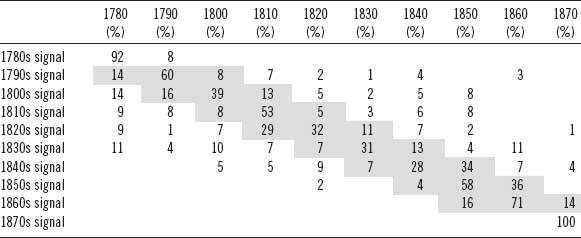
Note: Columns represent the actual decades of composition, and rows represent the computed “signal” associated with the decade in the row label. Percentages in the cells show the proportion of attributions to the row signal in the column decade.

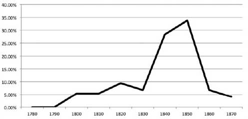
Figure 6.7. The 1840s signal over time

This phenomenon of successive generations, or waves, of style is visualized further in figure 6.8, where time is represented on the x axis, and the assignments are plotted as a percentage of all assignments in the given class on the y axis. Each shaded area represents a single decade's signal as it is detected across the entire one hundred years of the data set. The signals, like ripples in a pond of prose, peak chronologically from left to right. Ninety percent of the 1780s assignments appear in the 1780s. The remaining 10 percent (not visible behind the other areas in the chart) are assigned to text segments from the 1790s. The second-to-last signal in the chart, the 1860s signal, is first seen in the 1850s, with 16 percent of all the assignments to this signal, followed by 71 percent in the 1860s and then 14 percent in the 1870s. The data appear to confirm Moretti's observation that literary genres evolve and disappear over roughly thirty-year generations. Remember, however, that Moretti is speaking specifically of genre. Here we are not tracking genre signals at all; we are tracking decade signals. Or are we?

If we look at the distribution of novels in the corpus based on their genres and decades of publication, we see something similar to the generations discovered in the plotting of the stylistic “decade” signals. Table 6.4 shows the composition of the full corpus of 106 novels in terms of genre and decade: percentages are calculated by row and represent the proportion of texts from a genre (noted in the row label) that was published in a specific decade column. For example, the first row tells us that 15 percent of the Gothic novels in the corpus were published in the 1780s.

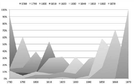
Figure 6.8. Generational waves of genre

Table 6.4. Distribution of novel genres over time

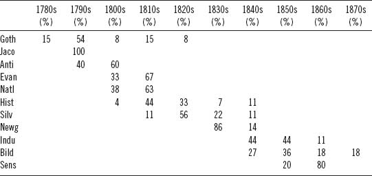
Table 6.4 is thus similar to Moretti's representation of genre in figure 9 of Graphs, Maps, Trees (2005), but with the addition here of percentages to represent the distributions of texts in our particular test corpus. No statistics are required to see that there is an obvious linear correlation between time and genre.* Nor is it too surprising to discover this given that the genre designations were probably assigned, at least in part, to help delineate the texts by period. The open question remains unanswered: are the “signals” that the model constructed to identify decades in fact stylistic manifestations of genre? The answer turns out to be no, but no with enough caveats and qualifications that in the absence of further data, one might argue the contrary.

Notice in table 6.4 how in every decade, except for the 1780s and 1870s, at least two genres are represented. In the 1800s column, for example, there are five genres. The same is true for the 1840s. Excepting the 1780s and 1870s, the stylistic signal of each decade in the model is constructed from a sampling of texts covering at least two and up to five different genres. It cannot, therefore, be asserted that the decade model the algorithm produced is really just a genre model in disguise—each decade signal is constructed from a sample of more than one genre. It is a complicating factor that genres are not confined to single decades; they bleed into subsequent and prior decades.

To better understand how the decade model in this experiment is generated, it is instructive to see the distribution of texts in each decade broken down by genre. Table 6.5 provides such a breakdown. Unlike table 6.4, where percentages are calculated to show distributions of each genre across all of the decades, table 6.5 shows the distribution of genres within each decade as a percentage of all works in a given decade. In other words, the percentages in table 6.5 are calculated according to the decade columns (adding up to 100 percent), whereas in table 6.4 it was the rows that totaled 100 percent. Table 6.5 allows us to see the raw, generic material upon which the model builds its “picture” of a given decade. The decade signal the model builds for the 1790s, for example, is composed of five parts Jacobin texts, four parts Gothic, and one part anti-Jacobin. Only the signals created for the 1780s and 1870s are “pure” in terms of being constructed of material from a single genre: the former composed entirely of Gothic texts and the latter of Bildungsroman.

To probe this evolving and complex chicken-versus-egg phenomenon, it is necessary to chart the presence (and absence) of the various genre signals over the course of time as a form of comparison. In other words, we must build a model sensitive to generic differences and then chart the resulting genre assignments over time. Regardless of whether the classifier's assignment is correct, we assume that the “signal” it has constructed is correct. Doing so allows us to track the signals that are characteristic of each novel's genre style and then to plot the manifestations of these signals over the course of the century.

Figure 6.9 provides an adequate if somewhat impoverished way of visualizing the presence of genre signals over time. Keep in mind that the data being plotted here come not from the actual human-identified genres of the novel but rather from the genre signals that the model has detected, regardless of whether the model is “correct.” To make the chart easier to read, I have ordered the genres in a way that maximizes the visibility of each data series. From this graphic, we may conclude that at least some genre signals exist as generations, and at least in these data the genres that exhibit the thirty-year generations that Moretti hypothesized tend to be what we might call the “minor” genres. The anti-Jacobin signal, for example, is clearly operative for just three decades, 1780–1810. So too with the Jacobin signal, which is expressed from 1790 to 1820. Less generational are the industrial, historical, and Gothic signals. The industrial signal spans nine decades, with a brief hiatus from 1800 to 1810. The historical signal begins in the 1780s and then persists for seven decades. The Gothic signal operates for six decades, beginning in the 1780s. The most befuddling signal is that derived from the silver-fork novels. The silver-fork signal, though never very strong, covers the entire period from 1790 to 1859, seven decades. The silver-fork novels in this corpus derive primarily from the 1820s (five novels) and 1830s (two novels). There is one each from the 1810s and 1840s. The signal is, however, more widely and more evenly (in terms of variance) distributed across the century than any of the other signals.*

Table 6.5. Genre composition by decade

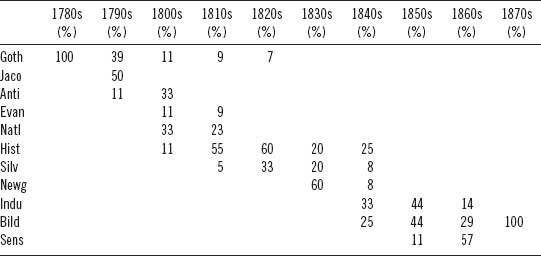
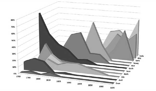
Figure 6.9. Genre signals over time

Returning to the probability data for the assignments reveals that of all the genre signals, the silver-fork signal is the weakest in terms of distinguishing itself. In other words, because so few features truly define the silver-fork class and set it apart from the other genres, it rarely manages to score very high in terms of probability over the other classes. In short, the silver-fork signal just is not distinctive; it is, compared to the other eleven genres, relatively bland and average. As a result of its weak signal, those cases where silver-fork is selected as the most likely class are often cases with only a slight edge over another competing genre. In one classification test, for example, 27 of 354 test segments were assigned to the silver-fork genre, yet, of those 27, only 5 (19 percent) were considered to have a probability greater than 90 percent. In the same test, 46 out of 55 (84 percent) Gothic novels were considered to have a probability above 90 percent. That the Gothic is more easily detected than the silver-fork is clear, but why?

Put to the side, for a moment at least, what we know about the silver-fork as a genre (that is, that it was a genre of novels about the fashionable life of the upper class typically penned by writers of the middle class who—at least according to William Hazlitt—knew not of what they wrote) and consider simply the linguistic features that distinguish the Gothic and silver-fork novels. In the top-ten words most important to distinguishing the Gothic from the other eleven genres, we find upon, from, by, and where all frequently used. Least important to the Gothic is the apostrophe followed by quotation marks, which are, naturally, indicative of dialogue. In total, there are forty-eight features that clearly identify the Gothic novel by either their presence or their absence.* The silver-fork, on the other hand, offers only six such distinguishing features. Standout features in the silver-fork genre include an above-average use of the semicolon; the words even, too, how, and ever; and the single underutilized word father. Obviously, the classifier uses more than these six (or even forty-eight) words in its calculations, but drawing attention to these “highly indicative” features gives some insight into the comparative difficulty the learning algorithm will have in building a signal for each class.

Although the classifier has no knowledge of genre, or even of the meanings of words themselves, it is instructive to use our human knowledge to understand or even interpret the classifier's discoveries. Among the words that best define the Bildungsroman, the top three are the words like, young, and little.† The significance of young to the Bildungsroman genre seems obvious enough: these are novels about development into adulthood. And little, an adjective describing youth and size, is an unsurprising term to find prominently in a novelistic genre that deals with maturation and growth from childhood. Like, on the other hand, is a word expressing resemblance or comparison. Here a move in the direction of close reading is warranted and informative. A closer look at several Bildungsroman texts in the corpus reveals that like frequently occurs in scenes in which a protagonist is seen discovering a new adult world and is using like as a means of comparison to the more familiar child's world. Young David Copperfield, for example, frequently employs like to bring the larger world around him into terms that his child's sensibility is able to comprehend: for example, “As the elms bent to one another, like giants who were whispering secrets…” (Dickens 1850, 4). Like also appears frequently in places where Copperfield seeks to make sense of the adult world around him, as in the following examples: “Mr. Chillip laid his head a little more on one side, and looked at my aunt like an amiable bird” (ibid., 9). “She vanished like a discontented fairy; or like one of those supernatural beings, whom it was popularly supposed I was entitled to see” (ibid.). “If she were employed to lose me like the boy in the fairy tale, I should be able to track my way home again by the buttons she would shed” (ibid., 20). “Opposite me was an elderly lady in a great fur cloak, who looked in the dark more like a haystack than a lady” (ibid., 52). Not surprisingly, as the narrative progresses, and Copperfield ages, the usage of like diminishes. Figure 6.10 shows the distributions of like and little over ten equal-size chunks of the novel. The y axis is the relative frequency of the terms and the x axis the course of the novel from beginning to end. Linear trend lines (dashed) have been added to each data series. Similar patterns for different word types can be found among the other genres as well. Newgate novels, which glamorize the lives of criminals, show a disproportionate fondness for the exclamation point and a disproportionately low usage of the female pronouns and honorifics she, her, and miss. Both Jacobin and anti-Jacobin novels tend to favor first-person pronouns with a high incidence of my, me, myself, and I, but in anti-Jacobin novels more feminine words are found, words such as her, lady, and Mrs., which are all negatively indicated for the Jacobin novel.

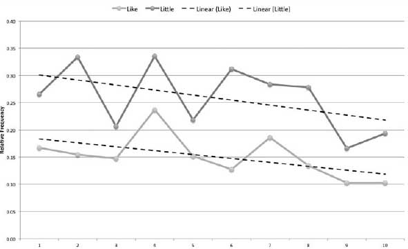
Figure 6.10. Distribution of like and little in David Copperfield

Industrial novels, more than any other genre in the collection, favor the use of the possessive. These are novels about possessions: what is “mine” versus “yours,” that which belongs to the rich and that which the poor aspire to have. But the industrial novel also favors the use of the conditional if: a word representing both possibility and contingency, a word that can effectively express juxtaposition and call attention to antithesis. Describing Coketown, Dickens writes in Hard Times, “It was a town of red brick, or of brick that would have been red if the smoke and ashes had allowed it” (1854, 26). Here if serves to overturn expectation with reality, first to set up and then to undermine. The overall effect is one that highlights and calls attention to the less than ideal realities of the working class. At first the narrator sees redbrick—that is, after all, what buildings are made of. So commonplace is this sight that at first the narrator fails to see what the bricks have become in the realities of Coketown. Some pages later, writing more specifically about the Coketown working class, Dickens again employs if to dramatic effect: “among the multitude of Coketown, generically called ‘the Hands,’—a race who would have found more favour with some people, if Providence had seen fit to make them only hands, or, like the lower creatures of the sea-shore, only hands and stomachs” (ibid., 75). Unlike the former example in which if is used as a corrective to a reader's (and the narrator's) expectations, here if dramatizes the helplessness of the workers who would have been better liked if only they had been not people, but mere “hands,” some form of primitive organism capable only of fulfilling some simple task.

In Mary Barton, Elizabeth Gaskell allows John Barton to address similar matters in an even more direct way. Here if is employed repeatedly and dramatically to contrast the differences between the rich and the poor:

“And what good have they ever done me that I should like them?” asked Barton, the latent fire lighting up his eye: and bursting forth, he continued, “If I am sick, do they come and nurse me? If my child lies dying (as poor Tom lay, with his white wan lips quivering, for want of better food than I could give him), does the rich man bring the wine or broth that might save his life? If I am out of work for weeks in the bad times, and winter comes, with black frost, and keen east wind, and there is no coal for the grate, and no clothes for the bed, and the thin bones are seen through the ragged clothes, does the rich man share his plenty with me, as he ought to do, if his religion wasn't a humbug? When I lie on my death-bed, and Mary (bless her) stands fretting, as I know she will fret,” and here his voice faltered a little, “will a rich lady come and take her to her own home if need be, till she can look round, and see what best to do? No, I tell you, it's the poor, and the poor only, as does such things for the poor. Don't think to come over me with th’ old tale, that the rich know nothing of the trials of the poor, I say, if they don't know, they ought to know. We're their slaves as long as we can work; we pile up their fortunes with the sweat of our brows; and yet we are to live as separate as if we were in two worlds.” (1849, 10–11)

These examples underscore how the micro scale (that is, close reading) must be contextualized by the macro scale: genres do have distinct ways of employing linguistic features, and unless we bring these distinctions to consciousness, we risk misinterpretation. So genres can be detected algorithmically with a fair degree of precision. In and of itself, this is not especially useful. Although with a good genre detector in place we could imagine mining the “great unread” in search of new texts that possess a specific, or even “preferred,” signal, it is more interesting to consider what this discovery means in terms of authorial freedom and how novels actually get written, to draw the inevitable connections between content, form, and style. A writer wishing to produce a novel of a certain genre, of a certain type, is bound, either consciously or unconsciously—and I believe it to be more of the latter than the former—by the conventions of linguistic usage that are endemic to that form.

Previously, we have thought of these conventions in terms of plot: a Bildungsroman involves the protagonist's maturation; a Newgate novel involves a criminal's exploits. But with these plot conventions come stylistic constraints, constraints that determine the very vocabulary an author has to work with. These constraints exist at the level of the most common linguistic features. The “feel” of a piece of writing, its “style,” is made manifest through the type and variety of common words and marks of punctuation that a writer deploys. But it is the “big” words writers agonize over, not the little ones. Should the sunset be described as beautiful or magnificent? Beautiful and magnificent, these are the class of words that we use with care and reservation. The little words—the, of, it—are engaged automatically, spontaneously. These little words fall outside of deliberate, conscious control, much like the tics of a poker player who gives away his hand by a telling twitch or sigh. We know this to be true: authors have these idiosyncrasies. An analysis of the Federalist Papers—a corpus in which context, genre, gender, and historical time are all held constant—reveals that Hamilton prefers using a more than Madison and Jay, but he uses the conjunction and less often than Madison and far less often than Jay. And Hamilton prefers the infinitive to be over Jay and Madison, whose preference swings toward is. Subtle peculiarities of word usage offer telling signals of genre, but are even more telling of their makers. These subtle habits give authors away, but they do so in ways that only a machine is likely to detect.

At least under normal circumstances, we can assume that the author of Hard Times really is Charles Dickens, that Charles Dickens really is a male author, and that any randomly selected chunk of text from Hard Times really is a chunk of text from the novel Hard Times by the male author Charles Dickens. Unsurprisingly, the classification data show quite clearly that the better a category is defined, the better the classifier can detect and build a signal upon it. In other words, classifications based on loosely defined genres produce comparatively poor results when viewed next to the results for a more objectively defined category such as gender or author. Despite the presence of forty-seven different authors in this test corpus, the model was able to detect enough variation between author signals to correctly identify the authors of a random set of samples with 93 percent accuracy. This may feel uncomfortable, even controversial, to those reared in the “there is no author” school of literary criticism. The data are undeniable. Ultimately, it does not matter if Dickens is really Dickens or some amalgamation of voices driven to paper by the hand of Dickens. The signal derived from 161 linguistic features and extracted from books bearing the name “Charles Dickens” on the cover is consistent.

The strength of the author signals in this experiment in fact trumps the signals of individual texts—something intuition does not prepare us for.* The classifier is more likely to identify the author of a given text segment than it is to correctly assign that same text segment to its novel of origin. What ultimately separates one Jane Austen novel from another is not linguistic style but subject matter. Austen, in fact, has one of the most consistent and unvaried styles of all the writers in this corpus. No offense to Austen fans intended, but Jane is easy to detect—her style is, as it were, an open book. Prose by a writer such as Mark Twain or James Joyce, on the other hand, is extremely hard to quantify and then detect because the works of these two writers demonstrate a much greater stylistic range. Their range makes the development of a stable signal far more difficult.

Before coming to that analysis, however, it is worth unpacking what happens with author gender. A gender signal was evident, and at 80 percent accuracy it is a strong signal, if still comparatively weak next to the author signal. This overall rate of accuracy is consistent with the conclusions of Moshe Koppel, Shlomo Argamon, and Anat Rachel Shimoni, who demonstrate that “automated text categorization techniques can exploit combinations of simple lexical and syntactic features to infer the gender of the author of an unseen formal written document with approximately 80 per cent accuracy” (2002, 401). The feature data from my gender classification experiment show that female authors are far more likely to write about women, and they use the pronouns her and she far more often than their male counterparts.† In fact, these are the two features that most distinguish the male and female authors in this corpus. The females in this data set also show a preference for the colon and the semicolon, which are the third and fourth most distinguishing features. Not surprisingly, it is also seen that women authors show higher usage of the words heart and love—not surprising in the sense that this fact is consistent with our stereotypes of “feminine” prose. Nevertheless, there are the features that contradict our stereotypes: male authors in this corpus are far more likely to use marks of exclamation, and women are not the primary users of we and us, despite what some may think about which is the more conciliatory gender. Table 6.6 provides an ordered list of the features most influential in distinguishing between the male and female authors in this corpus. The parenthetical M/F indicates which gender has a higher use pattern for the given term, and the P indicates a punctuation feature.

Faced with this evidence and the prior work of Koppel, it is hard to argue against the influence of gender on an author's style. Although there may be some genres of prose in which these signals become muted—in legal writing, for example—when it comes to the nineteenth-century novel, it is not terribly difficult to separate the men from the women. Far more interesting than this revelation, however, is an examination of which authors get misclassified as being of the other gender. Table 6.7 provides a list of all the authors who received misattributions and how often.

Table 6.6. Features best distinguishing male and female authors

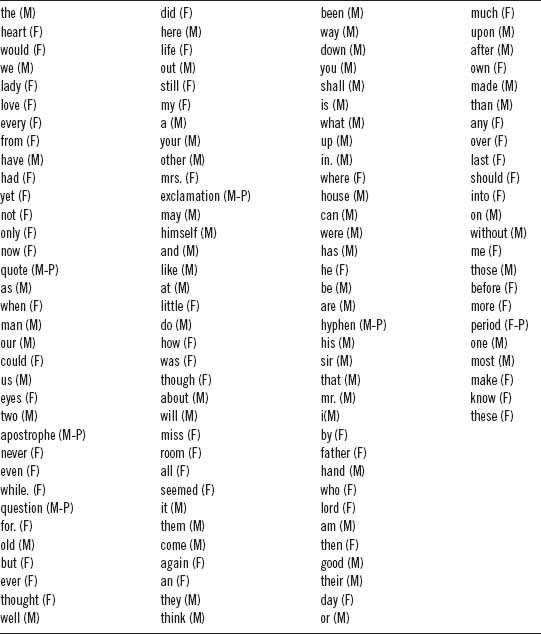
Table 6.7. Misattribution of gender

Author	Percentage error
Mary Elizabeth Braddon	50.00
William Beckford	40.00
George Eliot	33.33
M. G. Lewis	30.00
John Moore	30.00
Robert Bage	20.00
William Godwin	20.00
Ann Thomas	20.00
Maria Edgeworth	17.50
Catherine Gore	15.00
Lady caroline Lamb	10.00
Edward Lytton	10.00
Lady Morgan	10.00
Anthony Mope	10.00
Anna Marie Porter	5.00
Ann Radcliffe	5.00
Benjamin Disraeli	3.33
John Galt	3.33
Walter Scott	3.33
Charlotte Brontë	2.50

Mary Elizabeth Braddon has the distinction of being the most androgynous writer in the corpus, with 50 percent of her segments being classed as male. William Beckford is next, with 40 percent of his segments being labeled as female. The greatest number of raw misclassifications goes to George Eliot, an interesting distinction for a female author who wrote under a male pseudonym. Ten out of thirty samples from Eliot are incorrectly attributed to the male signal. Of the ten, six are from Middlemarch, three from Felix Holt, and one from Daniel Deronda. The remaining authors were “outed” fairly easily—convincing evidence, to be sure, that authors are not above the influences of their gender.

Where author and gender were easy to detect, detecting genres and time periods presented an especially challenging situation. These two are challenging because they are deeply interconnected but also because they are constructed upon arbitrary distinctions. Genres are a subjectively derived and human-defined classification system in which boundaries are primarily drawn in terms of subject matter. Genre boundaries are notoriously porous, and genres bleed into each other.* Decade is even more arbitrary. Decades are simple chunks of time in an infinite continuum. Even years are arbitrary—if a bit less arbitrary than decades since books happen to be published in years, but arbitrary all the same since books get written and then published in different years.† Nevertheless, some interesting facts about genres and time periods are made manifest by this analysis. It turns out that to write a Gothic novel, an author inevitably ends up using more positional prepositions than if writing a Bildungsroman. If a writer is employing a few too many exclamation points, it is more likely that either she is a he or that he/she is writing a Newgate novel rather than a more comma-heavy historical novel. Even though context-sensitive words have been intentionally excluded from this analysis, there is most certainly some correlation between subject and frequent word usage. That said, there is evidence too that subject matter is only part of the equation; the author, gender, and text-based signals are incredibly strong. At least some genres are, or appear to be, generational in nature. This is especially true of the “minor” genres. Where genre signals break down, time-oriented signals step in, revealing cycles of style that, though at times appearing to connect with genre, also transcend genre and suggest the presence of a larger stylistic system.

• • •

Despite strong evidence derived from this classification analysis, further verification of these tendencies was warranted. To take the analysis one step further, I constructed a second test using linear regression to model and measure the extent to which each of the five “external” variables (text, author, genre, decade, and gender) accurately predicts the dependent variables (that is, the usage of frequent words and marks of punctuation). Linear regression is a statistical technique that is used to “fit” a predictive model to an observed data set. Given any one of the five categories, linear regression can be employed to quantify the strength of the relationship between the category and the individual linguistic features in the data set. Once the models are constructed, the statistical “F-test” may then be employed to compare the models in order to ascertain which of the models best fit the overall data. The F-test provides a measure of statistical probability in a “p-value,” and the p-value shows how strongly the features in the model predict the outcome. A small p-value indicates a feature that is strongly predictive of the outcome.

In this experiment, 5 by 161 linear models were fit, and p-values for each were calculated. The resultant p-values for each of the 161 variables within each of the five categories were then tabulated such that each column represented one of the five categories (author, genre, and so on) and each row one of the 161 linguistic features. The resulting cells contained the corresponding p-value for a given dependent variable in a category. For each of the 161 dependent variables, the smallest of the five corresponding p-values reveals which of the five external variables is most predictive of the dependent variable. In other words, it is possible to determine whether it is the author, the text, the genre, the decade, or the gender that best explains or predicts the behavior of each one of the 161 linguistic variables. The p-values can then be tabulated and ranked for each column so as to arrive at a single value representing the estimated percentage of “influence” that each category exerts on the final linguistic product.

With minor exceptions, the results of this linear regression analysis confirmed what was seen in the machine-classification experiment described above. The only difference is that in this secondary analysis, the strengths of the “author” and “text” signals were reversed: here the text was seen to be the strongest predictor of the linguistic features. Figure 6.11 provides a percentage-based view of the relative influence of each factor in the overall linguistic signal captured by the 161 variables.

For all but 17 of the 161 variables, text was the strongest predictor of usage. Next strongest was author, followed by genre, then decade, and finally gender. Plotting all five categories on a stacked bar chart (figure 6.12) allows for visualization of the relative strength of each feature within each category. Working from the bottom of the chart upward, the text (black) and author (dark gray) signals dominate the chart, followed by genre, decade, and gender (in very light gray).

Even more interesting than these overall trends, however, are the ways in which specific features appear to be tied to specific categories. The gender signal is by far the least important, but gender does have greater influence on some variables than others. Confirming the results from the classification tests explored above, the linear regression test identified the two variables most determined by gender as her and she. Heart and love follow closely behind.* Again, as was seen in the classification tests, when it comes to the author signal, the linguistic features that have the greatest importance are not words, but marks of punctuation. In the linear regression test, six of the top eight variables that are most easily predicted by author are marks of punctuation: the comma is first, followed by the period in fourth place, the colon in fifth, semicolon in sixth, and hyphen in eighth. With genre, we find an overwhelming presence of prepositions as top predictors, particularly locative prepositions including, in order, to, about, and up. Also in the top ten are come and there, two more words indicative of location or “scene-setting” language and two words that showed up as important in the other method as well. Also found are the previously discussed words like and little, which we know to be of particular importance in distinguishing the Bildungsroman from other genres.

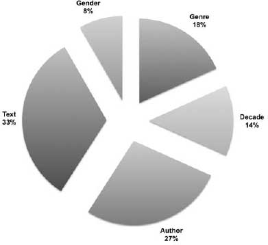
Figure 6.11. Percentage view of category influence

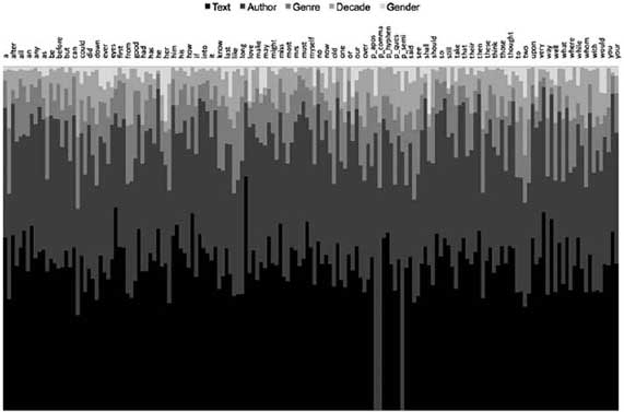
Figure 6.12. Relative view of category influence

• • •

Some micro thoughts…Claudi Guillén writes in Literature as a System that “genre is an invitation to form” (1971, 109). To “form” we must certainly now add “style,” or if style is too broad a term for some tastes, then at the very least we must add “language usage.” The data presented here provide strong evidence for existing notions of individual authorial “fingerprints,” but show further that author signal alone does not account for the variance in the linguistic data. No doubt, a good share of the variance may be attributed to the particular text that the author is writing, and since the text belongs to, is the creation of, an author, it may be right to conflate the author and text signals into one piece of the pie. Having done so, however, we still have another half pie to account for. Both the classification tests and the linear regression tests showed gender to be a bit player. This was especially evident in the linear regression, where gender rises to only 8 percent of the influence. Even when the classifier showed strong accuracy (at 80 percent), it was still magnitudes below the other categories in terms of improvement over chance. Time and genre are clearly the most complicated factors to understand and thus the most interesting to pursue. It is clear that an author's choice of genre plays a role in determining the subject and form that a novel takes, but genre also plays a role in determining the linguistic material from which the content is derived. Some genre forms clearly move writers to employ more prepositions; other genres demand more articles, or more pronouns, and so on. Given the powerful influence of the author signal and the less powerful but still important factors of time and gender, it is difficult to go much further at the macroanalytic scale. What is required to probe the strength of genre further is an environment in which we can control for gender, author, and time and thus truly isolate the genre signal. In short, we need Charles Dickens, Edward Lytton, and Benjamin Disraeli.

These authors are useful because they are all represented in the test corpus, and they share the distinction of each having authored novels in at least three different genres. From Dickens, the test corpus includes one Bildungsroman, one industrial novel, and one Newgate novel; from Lytton, there is one historical novel, one Newgate novel, and one silver-fork novel; from Disraeli, there is one Bildungsroman, one industrial novel, and one silver-fork novel. Before analyzing the contributions from these three authors and five genres, I will begin by exploring a larger subset of my original corpus that includes just the authors of novels in the Bildungsroman and industrial genres. This allows for a rough approximation of how well the data separate according to genre. Using the same linguistic feature set employed previously, all of the text segments of Bildungsroman and industrial novels (two hundred segments from ten different authors) were isolated and compared. First, an unsupervised clustering of the data was used in order to determine whether the two genres would naturally cluster into two distinct categories. The results of the clustering (table 6.8) were inconclusive: ninety (81 percent) Bildungsroman segments clustered with forty (44 percent) industrial segments into one group and twenty (18 percent) Bildungsroman with fifty (56 percent) industrial into another.* In other words, though there was some separation, neither cluster was dramatically dominated by one genre or another. When the same data were grouped into ten clusters (there are ten authors in the data set who authored novels in either the Bildungsroman or the industrial genre), however, author clustering was quite apparent. Only one (Elizabeth Gaskell) of the ten authors had text segments assigned to more than two clusters. Table 6.9 shows the distribution of segment assignments by author and cluster.

In addition to the clustering analysis, principal component analysis was used to explore the data. In this test, the first two principal components accounted for 31 percent of the variance in the data, and like the clustering test, PCA revealed a good deal of overlap between the two genres (figure 6.13). Closer inspection of the PCA data, however, showed significant internal subclustering based on author (figure 6.14), confirming what was seen in the clustering analysis. In other words, in both tests, the author signal continued to overpower the genre signal.

Narrowing the field to include only data from the novels of Dickens, Disraeli, and Lytton continued to produce results in which the author signal dominated the clustering (figure 6.15). In this test, four novels from Dickens were isolated on the east side of the plot, away from the other two novelists, who are located to the west side of PC1. The three novels from Disraeli are separate from the four novels by Lytton on the north-south dividing axis of PC2.

Table 6.8. Clustering results for Bildungsroman and industrial

Cluster	1	2
Bildungsroman	90	20
Industrial	40	50

Table 6.9. Distribution of segment assignments by author and cluster

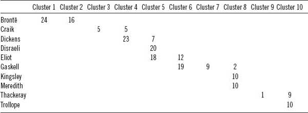
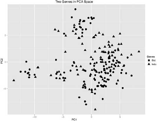
Figure 6.13. Bildungsroman and industrial novels in PCA space

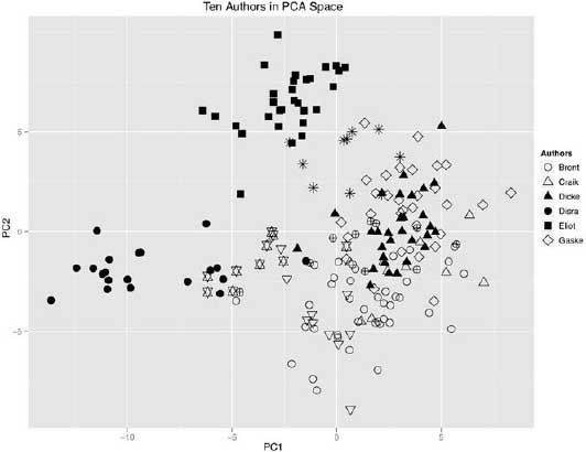
Figure 6.14. Ten authors in PCA space

What then of genre? What is not evident in figure 6.15 is that within each author cluster, there is further separation to be found and that the separation is largely attributable to genre. Figure 6.16 shows just the three novels of Disraeli: Coningsby, or, The New Generation (Bildungsroman); Sybil, or, The Two Nations (industrial); and Vivian Grey (silver-fork). PC1 and PC2 account for 53 percent of the variation in the data. Though the clustering here is not perfect, it is very close—one segment from Sybil appears in the Coningsby cluster and vice versa—and the misalignment of this one segment makes sense given the themes of the two books. Nevertheless, it could be argued that the separation seen here is just as easily attributable to the text signal, and perhaps more correctly so. We must therefore turn to Dickens, from whom we have four novels.

With Dickens a similar separation is seen by genre (figure 6.17), but in this case we see the two Bildungsroman novels (ten segments each from Copperfield and Great Expectations) cluster together in the northwest, all of the Newgate segments from Oliver Twist in the northeast, and Hard Times almost entirely in the south-central regions. In other words, the linguistic signals associated with the two Bildungsromans have more in common with each other than they do with the other non-Bildungsroman novels.

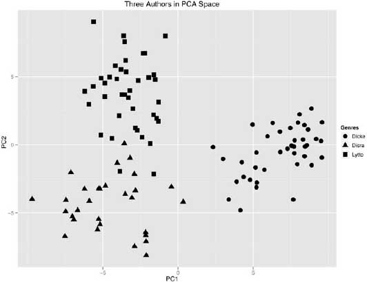
Figure 6.15. Three authors in PCA space

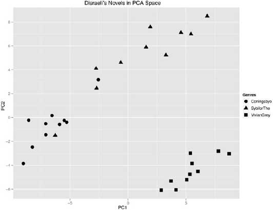
Figure 6.16. Disraeli's novels in PCA space

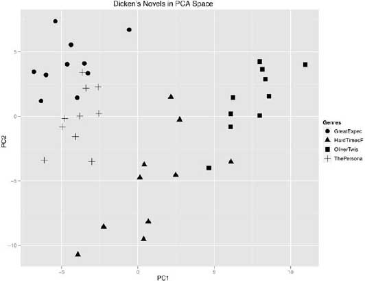
Figure 6.17. Dicken's novels in PCA space

Once we control for author, the full force of genre in this corpus can be seen. The linguistic choices that authors make are, in some notable ways, dependent upon, or entailed by, their genre choices. Having said that, additional experimentation has revealed—quite as we would expect—that not all genres exert equal force; some genres pull at style harder than others. Thought of in another way, some genres are more formal, more conventional. In this collection of data from twelve genres, the Bildungsroman holds the distinction of possessing the strongest signal, while Newgate novels contain a much more amorphous mixture of signals. The Bildungsroman has a stronger signal precisely because it is more formulaic, its conventions more clearly delineated. If form ever follows function, then style ever follows form.

---

* Even if the difference between the two finally boils down to a simple matter of opinion. One man's ore is another man's silt.

† How long Joyce spent picking the right words remains a mystery.

* These frequencies were derived from the plain text files archived at Project Gutenberg. File metadata were removed prior to processing.

† On the stealthy nature of pronouns, James W. Pennebaker's Secret Life of Pronouns offers an enlightening and entertaining perspective (2011).

‡ There are many ways in which a feature set may be derived, but the growing consensus is that the analysis of high-frequency words (mostly function, or closed-class, words) or n-grams, or both, provides the most consistently reliable results in authorship-attribution problems. See Burrows 2002; Diederich et al. 2000; Grieve 2007; Hoover 2003a, 2003b; Koppel, Argamon, and Shimoni 2002; Martindale and McKenzie 1995; Uzuner and Katz 2005; Yu 2008.

* Mick Alt provides an excellent, nontechnical, discussion of how PCA works in Exploring Hyperspace (1990).

† Jockers and Witten (2010) offer a benchmarking analysis of five high-dimensional, machine-learning algorithms for authorship attribution. See also Jockers, Witten, and Criddle 2008; Yu 2008; and a more extensive analysis in Zhao and Zobel 2005.

‡ Machine classification is employed extensively in what follows here and in subsequent chapters. A more extensive overview of the benefits will become apparent.

* This is a bit of a simplification; some of the papers are thought to have been coauthored. Details can be found in Mosteller and Wallace 1964.

* The decision to use 0.03 percent was arbitrary. The number was selected in order to ensure that the features were not context-specific words but function words that are used at a high rate. Zipf's law has demonstrated empirically that the frequency of any word in a corpus is inversely proportional to its rank in the frequency table. In other words, the frequency of the words drops off steeply.

† The forty-two words and punctuation features are as follows: a, all, an, and, as, at, be, but, by, for, from, had, have, he, her, his, I, in, is, it, me, my, not, of, on, p_apos, p_comma, p_exlam, p_hyphen, p_period, p_quote, p_semi, she, that, the, this, to, was, were, which, with, you.

‡ The mathematical details may be found by consulting the help files for the “dist” and “hclust” functions of the R statistical software package (http://www.R-project.org). Euclidean distance (“dist” in R) is explained in greater detail in chapter 9.

* The Nearest Shrunken Centroid classification algorithm (Tibshirani et al. 2003) was used in this experiment. A more detailed description of NSC follows below. The figure 33 percent represents the F-measure, or “F-score,” which is an aggregate measure of model accuracy.

† For example, there were only four evangelical novels, thus only forty fragment samples in the corpus upon which to train and test the model. The complete data set is available online at http://www.stanford.edu/group/litlab/cgi-bin/pamphletData/index.php?data_requested=one.

‡ Naturally, these human-assigned genres are not perfect. Scholars may in fact argue over whether any single novel is more appropriately placed in one genre or another, or perhaps, as is often the case, more than one. For this work, however, the selection of novels was done in a conservative fashion and in order to avoid novels that might be deemed too ambiguous.

* Remember too, that the texts have been segmented, so a particular segment could quite possibly be more “silver-forkey” than the novel as a whole.

* The 161 features selected were as follows: a, about, after, again, all, am, an, and, any, are, as, at, be, been, before, being, but, by, can, come, could, day, did, do, down, even, ever, every, eyes, father, first, for, from, go, good, great, had, hand, has, have, he, heart, her, here, him, himself, his, house, how, I, if, in, into, is, it, its, know, lady, last, life, like, little, long, lord, love, made, make, man, may, me, might, mind, miss, more, most, Mr., Mrs., much, must, my, myself, never, no, not, now, of, old, on, one, only, or, other, our, out, over, own, p_apos, p_colon, p_comma, p_exclam, p_hyphen, p_period, p_ques, p_quot, p_semi, room, said, say, see, seemed, shall, she, should, sir, so, some, still, such, take, than, that, the, their, them, then, there, these, they, think, this, those, though, thought, time, to, too, two, up, upon, us, very, was, way, we, well, were, what, when, where, which, while, who, whom, will, with, without, would, yet, you, young, your.

† A complete list of all the texts and their novelistic genres can be found in Allison et al. 2012.

* The analysis of style undertaken here is very similar if in fact a bit more complicated than this analogy might suggest.

† The NSC algorithms are available as part of the Prediction Analysis of Microarrays (pamr) package in the open-source R statistics software (R Development Core Team 2011).

* A centroid is the geometric center of a cluster of points.

† A layman's overview of how NSC works is available at http://www-stat.stanford.edu/~tibs/PAM/Rdist/howwork.html.

‡ Other classifiers could have been selected as well, but there was no reason to believe that one or another would be better suited to this problem than NSC. In separate research (Jockers and Witten 2010), it has been shown that five machine-learning algorithms performed well on this type of problem and that NSC was marginally better than the four other techniques tested.

§ A uniform prior was assumed on all classes during cross-validation.

¶ A 50 percent baseline for accuracy in binary classification is in fact true only in cases where there are an equal number of both classes in the test data. In the case of this experiment, it was very close to even: 52 percent of the test segments were from male authors and 48 percent from females.

# An examination of the confusion matrix, which is discussed below, indicates that the classifier does slightly better in classifying males versus females: 80 percent and 76 percent precision, respectively. Recall is slightly better for females, 79 percent versus 77 percent for males.

* In the above analysis, it was convenient to assume uniform prior probabilities for each class—if there are ten possible classes, then each class has a 10 percent likelihood of being selected by chance. In reality, the classes were never evenly distributed in this manner, and, thus, each class has a different baseline for accuracy. To fully explicate the results would require discussion of each class within each experiment. The confusion matrices (found online at http://www.matthewjockers.net/macroanalysisbook/confusion-matrices/) provide all the detail necessary for the reader to evaluate the results of these classification tests.

* Chronological stylistic change is explored in greater detail in chapter 9.

† We are reminded here of Harold Bloom's (1973) notion of “anxiety” as a motivation for change, of Colin Martindale's (1990) “law of novelty,” and of the Russian formalist Tynjanov's generational model of “archaists and innovators” in literary history.

* At least in this corpus of 106 novels, which was not constructed in order to be representative of novelistic variety or genre but rather as a way of exploring genre.

* The matter of finding atypical texts, or outliers within a given genre, is a problem worth probing. Students in my 2009 seminar discovered, for example, that Sir Walter Scott was a historical outlier in terms of the use of concrete diction versus abstractions. Scott, they argued, can thus be seen as a forerunner of a lexical tradition that is seen to develop in writers of later periods. The extent to which Scott can be viewed as the originator of this pattern is unclear, but it does seem that there are “evolutionary” forces at work. Scott may have been the first to develop this stylistic “mutation.” Whether the style that then persisted afterward was a result of a marketplace that preferred this style or whether later writers were consciously or unconsciously emulating Scott is a matter for future consideration. These questions are probed more deeply in chapter 9.

* Features that are overrepresented in Gothic novels include the words upon, eyes, still, from, by, now, were, these, where, had, himself, and he. Underutilized features include the apostrophe, the quotation mark, and the following words: lady, one, is, are, have, can, has, very, like, see, or, say, young, sir, little, know, good, own, as, think, well, make, us, two, must, house, made, do, take, man, come, Mr., if, and out.

† Other overutilized features of the Bildungsroman include the colon and the words made, when, thought, over, a, did, seemed, life, said, there, was, and then. Underutilized features include the words upon, by, your, may, the, and this.

* Most people, I think, would assume that it would be easier to assign a text segment to its originating text than to its author.

† Koppel's analysis also reveals the importance of gendered pronouns. Women tend to use feminine pronouns at a significantly higher rate than males.

* If you doubt this fact, spend a few hours trying to parse out the meaning in the publishing industry's BISAC codes.

† Serialized fiction presents an interesting case, and several students in the Stanford Literary Lab have been pursuing the question of whether serialization leads to any detectable differences in style. Students Ellen Truxaw and Connie Zhu hypothesize that the need to keep readers from one serial to the next puts stylistic demands upon writers and that these stylistic aberrations would be most apparent at the beginning and end of chapters and serial breaks. Truxaw and Zhu presented this work as “‘The Start of a New Chapter’: Serialization and the 19th-Century Novel” at the 2010 meeting of the International Conference on Narrative.

* A separate analysis of the usage of these terms in a larger corpus of 250 nineteenth-century British novels made available through Chadwyck-Healey shows that female authors use these terms at much higher rates than their male counterparts. See also Koppel, Argamon, and Shimoni 2002.

* Clustering was performed in R using the Distance Matrix Computation function (dist) and the Euclidean distance method. Hierarchical cluster analysis (hclust) was performed on the resulting distance object using the complete linkage method to determine similar clusters.