The PivotTable Wizard

Let us first walk through the PivotTable wizard to create our PivotTable. Then we will create the same PivotTable using code.

The first step is to select the source data and start the wizard by selecting PivotTable Report under the Data menu. This will produce the first wizard dialog, as shown in Figure 20-1. (These figures are for Excel 97 and 2000. The Excel XP wizard has a somewhat different appearance.)

Figure 20-1. Step 1 in the PivotTable wizard

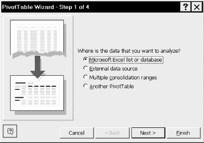
Note that this dialog allows us to select the data source for the PivotTable data. Clicking the Next button produces the dialog in Figure 20-2.

Figure 20-2. Step 2 in the PivotTable wizard

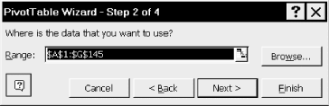
Since we selected the correct source range before starting the wizard, Excel has correctly identified that range in Figure 20-2, so we can simply hit the Next button, which produces the dialog in Figure 20-3.

Figure 20-3. Step 3 in the PivotTable wizard

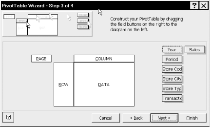
This dialog is where we format the PivotTable by deciding which columns of the original source table become pages in the PivotTable, which become rows, which become columns, and which become data (for aggregation). The procedure is to drag the buttons on the right to the proper location—row, column, page, or data. (We want one page for each of the two years.)

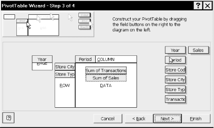
For our example, we drag the buttons to the locations shown in Figure 20-4. Note that the only button not used is Store Code. This field is the aggregate field, that is, we will sum over all store codes.

Figure 20-4. Step 4 in the PivotTable wizard

Clicking the Next button takes us to the dialog in Figure 20-5, where we choose the location for the PivotTable. We choose a new worksheet.

Figure 20-5. Step 5 in the PivotTable wizard

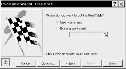
Clicking the Finish button produces the PivotTable in Figure 20-6.

Figure 20-6. The PivotTable

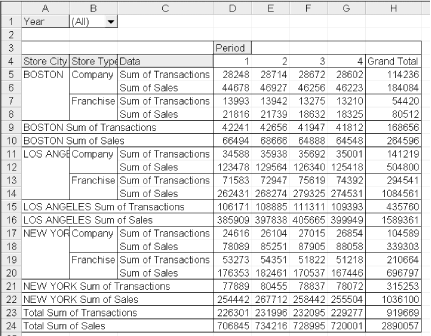
Note that the page button is labeled Year. Selecting one of All, 1998, or 1997 from the drop-down list box next to this button will confine the data to that selection. Thus, the pivot table has three pages: 1997, 1998, and combined (or All).

Note also that the columns are labeled by periods and the rows are labeled by both Store City and Store Type, as requested. In addition, Excel has created a new field called Data that is used as row labels. In this case, Excel correctly guessed that we want sums, but if Excel had guessed incorrectly we could make a change manually.

In summary, we can see that the main components of a pivot table are the pages, rows, columns, and data fields.

Rather than pursue further development of this PivotTable using the Excel interface, let us now switch to using code.