In previous chapters we introduced variable selection methods for selecting the correct submodel. We now present feature screening methods in which the goal is to discard as many noise features as possible and at the same time to retain all important features. Let Y be the response variable, and X = (X1, ⋯, XP)T consists of the p-dimensional predictors, from which we obtain a set of random sample {Xi,Yi}ni=1. The dimensionality p can be ultrahigh (i.e. the dimensionality p grows at the exponential rate of the sample n). Even though the variable selection methods introduced in the previous chapters can be used to identify the important variables, the algorithms used for optimization can still be very expensive when the dimension is extremely high. In practice, we may consider naturally a two-stage approach: variable screening followed by variable selection. We first use feature screening methods to reduce ultrahigh dimensionality p to a moderate scale dn with dn ≤ n, and then apply the existing variable selection algorithm to select the correct submodel from the remaining variables. This idea can also be employed iteratively. If all important variables are retained in the dimension reduction stage, then the two-stage approach is much more economical.
Throughout this chapter, we adopt the following notation. Denote Y =(Y1,,...Yn)T and X = (X1, ⋯ Xn)T, the n x p design matrix. Let Xj be the j-th column of X. Thus, X = (X1,... Xp). We slightly abuse notation X as well as Xi and Xj, but their meanings are clear in the context. Let ε be a general random error and ε= (ε1,...,εn)T with εi being a random errors. Let M, stand for the true model with the size s |M*|, and M̂ be the selected model with the size d=|M̂| The definitions of M, and M̂ may be different for different models and contexts.
8.1 Correlation Screening
For linear regression model (2.2), its matrix form is
 |
(8.1) |
When p > n, XTX is singular, and hence the least squares estimator of 0 is not well defined. In such a situation, ridge regression is particularly useful. The ridge regression estimator for model (8.1) is given by
where λ is a ridge parameter. As discussed in Chapter 3, the ridge regression estimator is the solution of penalized least squares with L2 penalty for the linear model. When λ → 0, then βλ tends to the least squares estimator if X is full rank, while λβ̂λ tends to XTY as λ →∞. This implies that β̂λ ∞ XTY when λ →∞.
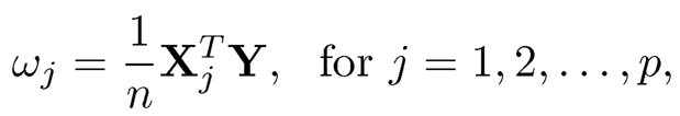
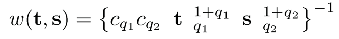
Suppose that all covariates and the response are marginally standardized so that their sample means and variances equal 0 and 1, respectively. Then 1/nXTY becomes the vector consisting of the sample version of Pearson correlations between the response and individual covariate. This motivates people to use the Pearson correlation as a marginal utility for feature screening. Specifically, we first marginally standardize Xj and Y, and then evaluate
 |
(8.2) |
which is the sample correlation between the jth predictor and the response variable.
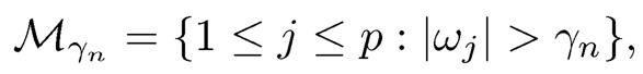
Intuitively, the higher correlation between Xj and Y is, the more important Xj is. Fan and Lv (2008) proposed to rank the importance of the individual predictor Xj according to |ωj| and developed a feature screening procedure based on the Pearson correlation as follows. For a pre-specified proportion ∈ (0, 1), the [γn] top ranked predictors are selected to obtain the submodel
 |
(8.3) |
where [γn] denotes the integer part of γn. It reduces the ultrahigh dimensionality down to a relatively moderate scale [γn], i.e. the size of M̂γ, and then a penalized variable selection method is applied to the submodel M̂γ. We have to set the value γ to carry the screening procedure. In practice, one may take the value of [γn] to be [n/ log(n)].
For binary response (coding Y as ±1), the marginal correlation (8.2) is equivalent to the two-sample t-test for comparing the difference of means in the jth variable. It has been successfully applied in Ke, Kelly and Xiu (2019) to select words that are associated with positive returns and negative returns in financial markets; see Figure 1.3.
8.1.1 Sure screening property
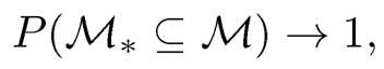
For model (8.1), define M*= {1 ≤ j ≤ p : βj # 0} with the size s Under the sparsity assumption, the size s should be much smaller than n. The success of the feature screening procedure relies on whether it is valid that M* ⊂ Mγ with probability tending to one.
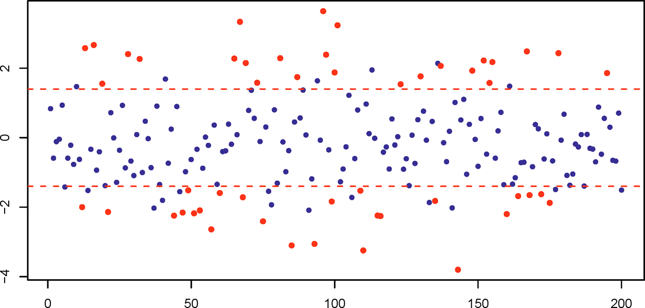
Figure 8.1: Illustration of sure screening. Presented are the estimated coefficients {β̂j}p j=1 (red dots are from M* and blue dots from Mc*. A threshold is applied to screen variables (|β̂j| > 1.5). Sure screening means that all red dots jump over bars. Blue dots exceeding the bars are false selections.
A variable screen or selection method is said to have a sure screening property if

Figure 8.1 illustrates the idea of sure screening. Fan and Lv (2008) proved that such a sure screening property holds with an overwhelming probability under the following technical conditions:
(A1) The covariate vector follows an elliptical contoured distribution (Fang, Kotz and Ng, 1990) and has the concentration property (See Fan and Lv (2008) for details about the concentration property.)
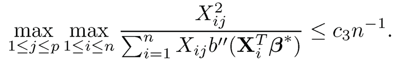
(A2) The variance of the response variable is finite. For some > 0 and c1, c2 >0, min 
(A3) For some τ ≥ 0 and c3 > 0, the largest eigenvalue of Σ = cov(X) satisfies λmax(Σ) ≤ c3nT, and ε ~N(0, σ2) for some σ > 0.
(A4) There exists a γ ∈(0,1 — 2k) such that log p = O(nξ), and p > n.
Theorem 8.1 Under Conditions (A1)-(A4), if 2κ + τ < 1, then there exists some 0 < θ <1 2k-τ such that when, -γ ~ cn-θ with c >0. Then for some C >0,
 |
(8.4) |
as n→∞.
This theorem is due to Fan and Lv (2008). It actually has two parts. Condition (A2) is the key to make the sure screening property (8.4) hold [even without condition (A3)]. Due to this property, the marginal (independence) screening procedure defined by (8.3) is referred to as sure independence screening (SIS) in the literature. It ensures that with probability tending to one, the submodel selected by SIS would not miss any truly important predictor, and hence the false negative rate can be controlled. Note that no condition is imposed on Σ yet. This is an advantage of the independence screening procedure. However, having the sure screening property does not tell the whole story. For example, taking M {1, ⋯, p}, i.e. selecting all variables, also has the sure screening property. That is where condition (A3) comes in to the picture. Under such a condition, the selected model size |M̂| =Op (n1-θ) is also well controlled. Therefore, the false positive rate is no larger than Op (n1-6/p), which is small when p > n.
The sure screening property is essential for implementation of all screening procedures in practice, since any post-screening variable selection method introduced in the previous chapters is based on the screened submodels. It is worth pointing out that Conditions (A1)-(A4) certainly are not the weakest conditions to establish this property. See, for example, Li, Liu and Lou (2017) for a different set of conditions that ensure the sure screening property. Conditions (A1)-(A4) are only used to facilitate the technical proofs from a theoretical point of view. Although these conditions are sometimes difficult to check in practice, the numerical studies in Fan and Lv (2008) demonstrated that the SIS can effectively shrink the ultrahigh dimension p down to a relatively large scale 0(n1-θ) for some θ > 0 and still can contain all important predictors into the submodel Mγ with probability approaching one as n tends to ∞.
8.1.2 Connection to multiple comparison
To illustrate the connection between the SIS and multiple comparison methods, let us consider the two-sample testing problem on the normal mean. Suppose that a random sample with size n was collected from two groups: Xi, i= 1, ⋯, n1 from the disease group, and Xi, i = n1 +1, ⋯, +n1 +n2= n from the normal group. Of interest is to identify which variables Xjs associate with the status of disease. For example, X consists of gene expression information, and we are interested in which genetic markers are associated with the disease. Such problems are typically formulated as identifying X3 with different means in different groups.
For simplicity, assume that Xi, ~N (μ1, Σ) for observations from the disease group, and Xi, ~N(μ2, Σ) for observations from the control group. Hotelling T2 (Anderson, 2003) may be used for testing H0 : μ1=μ2, but it does not serve for the purpose of identifying which variables associate with the
status of disease. In the literature of multiple comparison, people have used the two-sample t-test to identify variables associated with the disease status.
Denote x̄1j and x̄2j to be the sample mean for disease and normal groups, respectively. The two-sample t-test for H0j : μ1j = μ2j can be written as
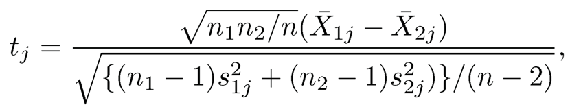
where s21j and s22j are the sample variance for disease and normal groups, respectively. Methods in multiple tests are to derive a critical value or proper thresholding for all t-values based on the Bonferroni correction or false dis- covery rate method of Benjamini and Hockberg (1995)(see Section 11.2 for further details) .
By marginally standardizing the data, assume with loss of generality that s21j =s22j =1 (by marginally standardizing). Then

As a result, ranking P-values of the two-sample t-test is equivalent to ranking |tj|, which is proportional to |X1j—X2j|. To see its connection with the Pearson correlation under linear model framework, define Yi= (1/n1)√n1n2/n if the i-th subject comes from the disease group, and Yi= -(1/n2) √n1n2/n if the i-th subject comes from the normal group. Then tj = XTjY. As a result, multiple comparison methods indeed rank the importance of variables in the two sample problem by using the sample Pearson correlation.
Fan and Fan (2008) proposed the t-test statistic for the two-sample mean problem as a marginal utility for feature screening. Feature screening based on co3 is distinguished from the multiple test methods in that the screening method aims to rank the importance of predictors rather than directly judge whether an individual variable is significant. Thus, further fine-tuning analysis based on the selected variables from the screening step is necessary. Note that it is not involved in any numerical optimization to evaluate ωj or XTY. Thus, feature screening based on the Pearson correlation can be easily carried out at low computational and memory burden. In addition to the computational advantage, Fan and Fan (2008) showed that this feature screening procedure also enjoys a nice theoretical property. Mai and Zou (2013) further proposed a feature screening procedures for the two-sample problem based on the Kolmogorov’s goodness-of-fit test statistic, and established its sure screening property. See Section 8.5.3 for more details.
8.1.3 Iterative SIS
The screening procedure may fail when some key conditions are not valid. For example, when a predictor Xj is jointly correlated but marginally uncorrelated with the response, then cov(Y, Xj) = 0. As a result, Condition (A2) is not valid. In such situations, the SIS may fail to select this important variable. On the other hand, the SIS tends to select the unimportant predictor which is jointly uncorrelated but highly marginally correlated with the response. To refine the screening performance, Fan and Lv (2008) provided an iterative SIS procedure (ISIS) by iteratively replacing the response with the residual obtained from the regression of the response on selected covariates in the previous step. Section 8.3 below will introduce iterative feature screening procedures under a general parametric model framework, to better control the false negative rate in the finite sample case than the one-step screening procedures. Forward regression is another way to cope with the situation with some individual covariates being jointly correlated but marginally uncorrelated with the response. Wang (2009) studied the property of forward regression with ultrahigh dimensional predictors. To achieve the sure screening property, the forward regression requires that there exist two positive constants 0 < τ1 < τ2 < ∞ such that τ1 < Amin(cov(X)) ≤ λmax(cov(X)) <τ2. See Section 8.6.1 for more details. Recently, Zhang, Jiang and Lan (2019) show that such a procedure has a sure screening property, without imposing conditions on marginal correlation which gives a theoretical justification of ISIS. Their results also include forward regression as a specific example.
8.2 Generalized and Rank Correlation Screening
The SIS procedure in the previous section performs well for the linear regression model with ultrahigh dimensional predictors. It is well known that the Pearson correlation is used to measure linear dependence. However, it is very difficult to specify a regression structure for the ultrahigh dimensional data. If the linear model is misspecified, SIS may fail, since the Pearson correlation can only capture the linear relationship between each predictor and the response. Thus, SIS is most likely to miss some nonlinearly important predictors. In the presence of nonlinearity, one may try to make a transformation such as the Box-Cox transformation on the covariates. This motivates us to consider the Pearson correlation between transformed covariates and the response as the marginal utility.
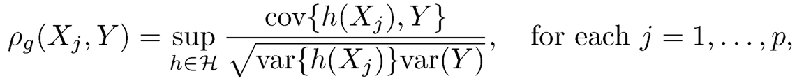
To capture both linearity and nonlinearity, Hall and Miller (2009) defined the generalized correlation between the jth predictor Xj and Y to be,
 |
(8.5) |
where H is a class of functions including all linear functions. For instance, it is a class of polynomial functions up to a given degree. Remark that if H is a class of all linear functions, ρg(Xj,Y) is the absolute value of the Pearson correlation between Xj and Y. Therefore, ρg(X, Y) is considered as a generalization of the conventional Pearson correlation. Suppose that {(Xij,Yi i = 1, 2, ..., n} is a random sample from the population (Xj, Y). The generalized correlation ρg(Xj,Y) can be estimated

where h̄j = n-1 Σni=1 h(Xij) and Ȳ = n-1 Σ ni=1 Yi. In practice, H can be defined as a set of polynomial functions or cubic splines (Hall and Miller, 2009).
The above generalized correlation is able to characterize both linear and nonlinear relationships between two random variables. Thus, Hall and Miller (2009) proposed using the generalized correlation ρg(Xj,Y) as a marginal screening utility and ranking all predictors based on the magnitude of estimated generalized correlation ρ̂(Xj, Y). In other words, select predictors whose generalized correlation exceeds a given threshold. Hall and Miller (2009) introduced a bootstrap method to determine the threshold. Let r(j) be the ranking of the jth predictor Xj; that is, Xj has the r(j) largest empirical generalized correlation. Let r* (j) be the ranking of the jth predictor X3 using the bootstrapped sample. Then, a nominal (1 — α)-level two-sided prediction interval of the ranking, [r̂_ (j), r̂+(j)], is computed based on the bootstrapped r*(j)’s. For example, if a = 0.05, based on 1000 bootstrap samples, r̂+(j) is the 975th largest rank of variable Xj. Hall and Miller (2009) recommended a criterion to regard the predictor Xj as influential if r̂+(j) < ½p or some smaller fraction of p, such as ¼ p. Therefore, the proposed generalized correlation ranking reduces the ultrahigh p down to the size of the selected model < kp}, where 0< k < 1/2 is a constant multiplier to control the size of the selected mode M̂k. Although the generalized correlation ranking can detect both linear and nonlinear features in the ultrahigh dimensional problems, how to choose an optimal transformation h(.) remains an open issue and the associated sure screening property needs to be justified.
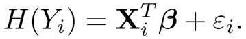
As an alternative to making transformations on predictors, one may make a transformation on the response and define a correlation between the transformed response and a covariate. A general transformation regression model is defined to be
 |
(8.7) |
Li, Peng, Zhang and Zhu (2012) proposed the rank correlation as a measure of the importance of each predictor by imposing an assumption on strict monotonicity on H(.) in model (8.7). Instead of using the sample Pearson correlation defined in Section 8.1.1, Li, Peng, Zhang and Zhu (2012) proposed the marginal rank correlation
 |
(8.8) |
to measure the importance of the jth predictor Xj. Note that the marginal rank correlation equals a quarter of the Kendall τ correlation between the response and the jth predictor. According to the magnitudes of all ωj's, the feature screening procedure based on the rank correlation selects a submodel
where γn is the predefined threshold value.
Because the Pearson correlation is not robust against heavy-tailed distributions, outliers or influence points, the rank correlation can be considered as an alternative way to robustly measure the relationship between two random variables. Li, Peng, Zhang and Zhu (2012) referred to the rank correlation based feature screening procedure as a robust rank correlation screening (RRCS). From the definition of the marginal rank correlation, it is robust against heavy-tailed distributions and invariant under monotonic transformation, which implies that there is no need to estimate the transformation H(·). This may save a lot of computational cost and is another advantage of RRCS over the feature screening procedure based on generalized correlation.
For model (8.7) with H(·) being an unspecified strictly increasing function, Li, Peng, Zhang and Zhu (2012) defined the true model as = {1 <j < p : βj #0} with the size s = |M*|. To establish the sure screening property of the RRCS, Li, et al. (2012) imposes the following marginally symmetric conditions for model (8.7):
(M1) Denote ΔH(Y) = H(Y1) — H(Y2), where H(·) is the link function in (8.7), and ΔXk = X1k — X2k. The conditional distribution FΔH-(Y)(Δxk(t) is symmetric about zero when k ∈ Mc*.
(M2) Denote Δεk = ΔH(Y) — ρ*kΔXk. Assume that the conditional distribution FΔεk|ΔXk(t)=π0kF0(t,σ20|ΔXk)+(1-π0k)F1(t,σ21)ΔXk follows a symmetric finite mixture distribution where F0(t, σ20|ΔXk) follows a symmetric unimodal distribution with the conditional variance σ20 related to ΔXk and F1 (t, σ21|ΔXk) is a symmetric distribution function with the conditional variance σ21 related to ΔXk when k ∈ M* π0k ≥ π*, where π* is a given positive constant in (0, 1] for any ΔXk and any k ∈ M.
Theorem 8.2 Under Conditions (M1) and (M2), further assume that (al) p = O(exp(nδ)) for some (δ ∈ (0, 1) satisfying (δ +2κ < 1 for any κ ∈(0, 0.5), (a2) assume min is a positive constant free of p, and (a3) the error and covariates in model (8.7) are independent. Then there exist positive constants c1, c2 >0 such that

Furthermore, by taking γn= c3n-κ for some c3 > 0 and assuming |pj|> cn-κ for j ∈ M„ and some c > 0, where ρi is the Pearson correlation between the response and the jth predictor.
 |
(8.9) |
This theorem is due to Li, Peng, Zhang and Zhu (2012) and establishes the sure screening property of the RRCS procedure. The authors further demonstrated that the RRCS procedure is robust to outliers and influence points in the observations.
8.3 Feature Screening for Parametric Models
Consider fitting a simple linear regression model
 |
(8.10) |
where ε*j is a random error with E(ε*j.|Xj) = 0. The discussion in Section 8.1.1 actually implies that we may use the magnitude of the least squares estimate β̂j1 or the residual sum of squares RSSj to rank the importance of predictors. Specifically, let Y and Xj both be marginally standardized so that their sample means equals 0 and sample variance equal 1. Thus, β̂̂j1 =n-1XTjY, which equals ωj defined in (8.2), is used to measure the importance of Xj. Furthermore, note that

as Xj is marginally standardized (i.e, ||Xj||2=n), and the least squares estimate β̂̂j0=Ȳ= 0. Thus, a greater magnitude of β̂̂j1, or equivalently a smaller RSSj, results in a higher rank of the jth predictor Xj. The same rationale can be used to develop the marginal utilities for a much broader class of models, with a different estimate of βj1 or a more general definition of loss function than RSS, such as the negative likelihood function for the generalized linear models. In fact, the negative likelihood function is a monotonic function of RSS in the Gaussian linear models.
8.3.1 Generalized linear models
Suppose that {Xi, Yi}ni=1are a random sample from a generalized linear model introduced in Chapter 5. Denote by

be the negative logarithm of (quasi)-likelihood function of Yi given Xi using the canonical link function(dispersion parameter is taken as ø= 1 without loss of generality), defined in Chapter 5 for the i-th observation {Xi Yi}. Note that the minimizer of the negative log-likelihood Σni=1 l(β0 + XTi β,Yi) is not well defined when p > n.
Parallel to the least squares estimate for model (8.10), assume that each predictor is standardized to have mean zero and standard deviation one, and define the maximum marginal likelihood estimator (MMLE) βj for the jth predictor Xj as
 |
(8.11) |
Similar to the marginal least squares estimate for model (8.10), it is reasonable to consider the magnitude of β̂ Mj1 as a marginal utility to rank the importance of Xj and select a submodel for a given prespecified threshold γn,
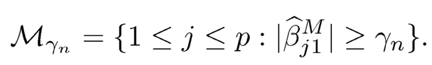 |
(8.12) |
This was proposed for feature screening in the generalized linear model by Fan and Song (2010). To establish the theoretical properties of MMLE, Fan and Song (2010) defined the population version of the marginal likelihood maximizer as

They first showed that the marginal regression parameters βMj1 = 0 if and only if cov(Y, Xj) = 0 for j = 1, … ,p. Thus, when the important variables are correlated with the response, βMj1 #0. Define the true model as M* = {1 ≤j ≤ p : βj #0} with the size s=|M*|. Fan and Song (2010) showed that under some conditions if

then

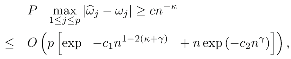
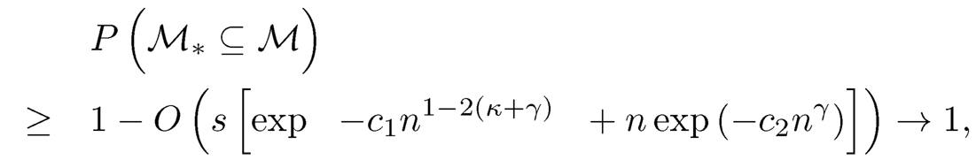
Thus, the marginal signals βMj1's are stronger than the stochastic noise provided that Xj ‘s are marginally correlated with Y. Under some technical assumptions, Fan and Song (2010) proved that the MMLEs are uniformly convergent to the population values and established the sure screening property of the MMLE screening procedure. That is, if n1-2κ/(k2nK2n)→∞, where kn= b'(KnB + B)+ m0Kan/ s0, B is the upper bound of the true value of βMi, m0 and s0 are two positive constants that are related to the model, and Kn is any sequence tending to ∞ that satisfies the above condition, then for any c3 > 0, there exists some c4 > 0 such that
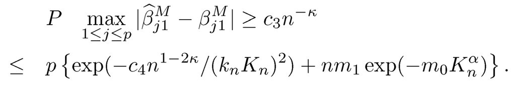
This inequality is obtained by the concentration inequality for maximum likelihood established in Fan and Song (2010). Therefore, if the right-hand side converges to zero (p can still be ultrahigh dimensional), then the maximum marginal estimation error is bounded by c3n-κ with probability tending to one. In addition, assume that |cov(Y, Xj)| ≥ c1n-κ for j ∈ M* and take γn = c5n-κ with c5 ≤ c2/2, the following inequality holds,
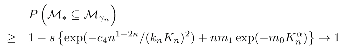 |
(8.13) |
as n → ∞. It further implies that the MMLE can handle the ultrahigh dimensionality as high as log p = o(n1-2κ) for the logistic model with bounded predictors, and log p = o(n(1-2κ)/4) for the linear model without the joint normality assumption.
Fan and Song (2010) further studied the size of the selected model M̂γn so as to understand the false positive rate of the marginal screening method. Under some regularity conditions, they showed that with probability approaching one, |Mγn|= O{n2κ λmax(Σ)}, where the constant determines how large the threshold γn is, and λmax (Σ) is the maximum eigenvalue of the covariance matrix Σ of predictors x, which controls how correlated the predictors are. If λmax(Σ) = O(nT), the size of Mγn has the order O(n2κ+τ).
The iterative feature screening procedure significantly improves the simple marginal screening in that it can select weaker but still significant predictors and delete inactive predictors which are spuriously marginally correlated with the response. However, Xu and Chen (2014) claimed that the gain of the iterative procedure is apparently built on higher computational cost and increased complexity. To this end, they proposed the sparse MLE (SMLE) method for the generalized linear models and demonstrated that the SMLE retains the virtues of the iterative procedure in a conceptually simpler and computationally cheaper manner. SMLE will be introduced in Section 8.6.2 in details.
8.3.2 A unified strategy for parametric feature screening
As discussed in the beginning of this section, one may use the RSS of marginal simple linear regression as a marginal utility for feature screening. The RSS criterion can be extended to a general parametric model framework.
Suppose that we are interested in exploring the relationship between X and Y. A general parametric framework is to minimize an objective function
 |
(8.14) |
where L(·,·) is a loss function. By taking different loss functions, many commonly-used statistical frameworks can be unified under (8.14). Let us provide a few examples under this model framework.
1. Linear models. Let L(Yi, β0+βTXi)=(Yi-β0-βTXi)2. This leads to the least squares method for a linear regression model.
2. Generalized linear models. Let L(Yi, β0+ βTXi) = Yi (β + XTi β) — b(β0 + XTi β) be the negative logarithm of (quasi)-likelihood function of Yi given Xi using the canonical link function(dispersion parameter is taken as 1 without loss of generality), defined in Chapter 5. This leads to the likelihood-based method for the generalized linear model, which includes normal linear regression models, the logistic regression model and Poisson log-linear models as special cases.
3. Quantile linear regression. For a given τ ∈ (0, 1), define ρτ(u) — u{α — I(u < 0)1, the check loss function used in the quantile regression (see Section 6.1), where I(A) is the indicator function of a set A. Taking L(Yi, β0 + βTXi) ρτ(Yi — β0— βTXi) leads to the quantile regression. In particular, τ = 1/2 corresponds to the median regression or the least absolute deviation method. As discussed in Section 6.1, quantile regression instead of the least squares method is particularly useful in the presence of heteroscedastic errors.
4. Robust linear regression. As discussed in Section 6.3, robust linear regression has been proved to be more suitable than the least squares method in the presence of outliers or heavy-tailed errors. The commonly-used loss function includes the L1-loss: ρ1(u) =|u|, the Huber loss function: ρ2(u) = (1/2)|u|2I(|u| ≤δ) + (δ{|u| — (1/2)δ}I(|ul >δ) (5) (Huber, 1964). Setting L(Yi, βTXi) =ρk (Yi - β0 +βT Xi), k=1 or 2 leads to a robust linear regression.
5. Classification. In machine learning, the response variable typically is set to be the input class label such as Y = {-1, +1} as in the classification method in the statistical literature. The hinge loss function is defined to be h(u) = {(1-u) + |1-u|}/2 (Vapnik, 1995). Taking L(Yi, β0 + βTXi) = h(Yi - β0 — βTXi) in (8.14) leads to a classification rule.
Similar to RSSj defined in the beginning of this section, a natural marginal utility of the jth predictor is
According to the definition, the smaller the value Lj, the more important the corresponding jth predictor. This was first proposed in Fan, Samworth and Wu (2009), in which numerical studies clearly demonstrated the potential of this marginal utility.
As mentioned in the end of Section 8.1.3, the marginal feature screening methodology may fail if the predictor is marginally uncorrelated but jointly related with the response, or jointly uncorrelated with the response but has higher marginal correlation than some important features. Fan, Samworth and Wu (2009) proposed an iterative screening and selection procedure (Iterative SIS) under the general statistical framework (8.14). The proposed iterative procedure consists of the following steps. We illustrate the idea in Figure 8.2.
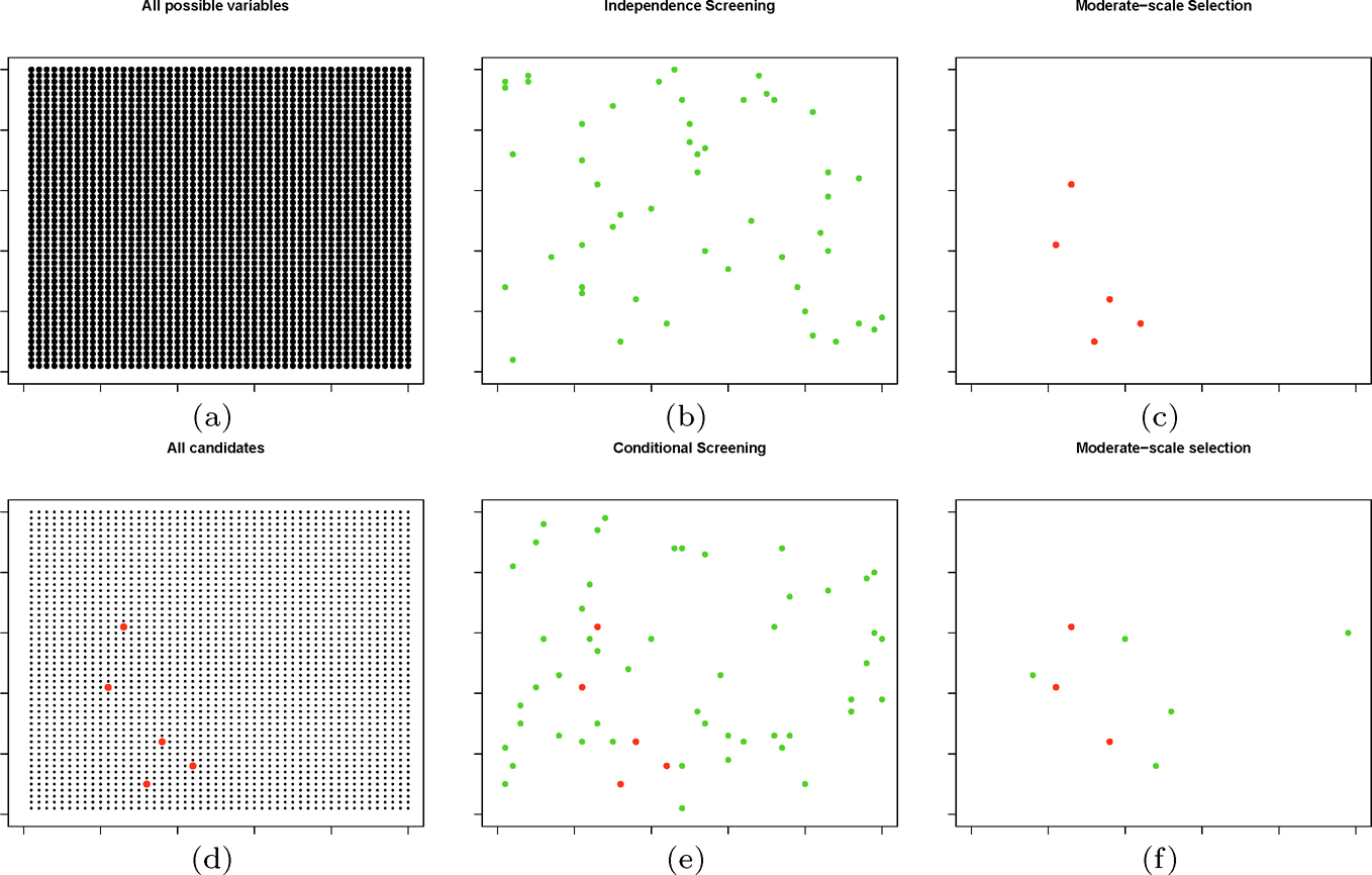
Figure 8.2: Illustration of iterative sure independence screening and selection. Starting from all variables (each dot in (a) represents a variable), apply an independence screening to select variables Â1 (green dots in (b)). Now select variables in (b) by applying a Lasso or SCAD and obtain the results (red variables M̂) in (c). Conditioning on red variables M̂ in (d) (the same as those in (c)), we recruit variables with additional contributions via conditional sure independence screening and obtain green variables A2 in (e). Among all variables M̂ U A2in (e), apply Lasso or SCAD to further select the variables. This results in (f), which deletes some of the red variables and some of the green variables.
S1. Compute the vector of marginal utilities (L1, …, Lp) (Figure 8.2(a)) and select the set Â1 = {1 ≤ j ≤ p : Li is among the first k1 smallest of all} (green dots in Figure 8.2(b)). Then apply a penalized method to the model with index set Â1, such as the Lasso (Tibshirani, 1996) and SCAD (Fan and Li, 2001), to select a subset M̂ (red dots in Figure 8.2(c)).
S2. Compute, for each j ∈ {1, ...,p}/M, the conditional marginal utility of variable Xj:
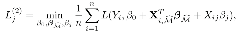
where Xi,M̂ denotes the sub-vector of Xi, consisting of those elements in M̂ (Figure 8.2(d)). L(2)j can be considered as the additional contribution of the jth predictor given the existence of predictors in M̂. Then, select, by screening, the set (green dots in Figure 8.2)
 is among the first k2 smallest of all}:
S3.Employ a penalized (pseudo-)likelihood method such as the Lasso and SCAD on the combined set M̂ ∪Â2 (green and red dots in Figure 8.2(3)) to select an updated selected set M̂. That is, use the penalized likelihood to obtain
where pλ(·) is a penalty function such as Lasso or SCAD. Thus the indices set of β̂2 that are none-zero yield a new updated set M̂ (green and red dots in Figure 8.2(f)).
S4.Repeat S2 and S3 until |M̂| ≤ d, where d is the prescribed number and d < n. The indices set M̂ is the final selected submodel.
This iterative procedure extends the Iterative SIS (Fan and Lv, 2008), without explicit definition of residuals, to a general parametric framework. It also allows the procedure to delete predictors from the previously selected set. Zhang, Jiang and Lan (2019) show that such a screening and selection procedure has a sure screening property, without imposing conditions on marginal regression coefficients and hence justifying the use of iterations.
In addition, to reduce the false selection rates, Fan, Samworth and Wu (2009) further introduced a variation of their iterative feature screening procedure. One can partition the sample into two halves at random and apply the previous iterative procedure separately to each half to obtain the two submodels, denoted by M̂(1) and M̂(2). By the sure screening property, both sets may satisfy P(M* ⊆ M̂(h)) →1, as n → ∈, for h=1, 2, where M* is the true model set. Then, the intersection M̂ = M̂(1) ∩M̂(2) can be considered the final estimated set of M. This estimate also satisfies that P(M* ⊆M̂) →1. This variant can effectively reduce the false selection rates in the feature screening stage.
8.3.3 Conditional sure independence screening
In many applications, one can know a priori that a set C of variables are related to the response Y and would like to recruit additional variables to explain or predict Y via independence screening. This naturally leads to conditional sure independence screening (CSIS). For each variable j ∈ {1, .. ,p}/C, the conditional marginal utility (indeed loss) of variable Xi is
Now rank these variables by using {Lj, j ∉ Cc}: the smaller the better and choose top-K variables.
Barut, Fan, and Verhasselt (2016) investigated the properties of such a conditional SIS. It gives the conditions under which that sure screening property can be obtained. In particular, they showed that CSIS overcomes several drawbacks of the SIS mentioned in Section 8.1 and helps reduce the number of false selections when the covariates are highly correlated. Note that CSIS is one of step (S2) in the Iterative SIS. Therefore, the study there shed some light on understanding the Iterative SIS.
8.4 Nonparametric Screening
In practice, parametric models such as linear and generalized linear models may lead to model mis-specification. Further, it is often that little prior information about parametric models is available at the initial stage of modeling. Thus, nonparametric models become very useful in the absence of a priori information about the model structure and may be used to enhance the overall modelling flexibility. Therefore, the feature screening techniques for the nonparametric models naturally drew great attention from researchers.
8.4.1 Additive models
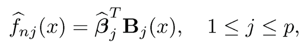
Fan, Feng and Song (2011) proposed a nonparametric independence screening (NIS) for the ultrahigh dimensional additive model
 |
(8.15) |
where {mj (Xj)pj=1 have mean 0 for identifiability. An intuitive population level marginal screening utility is E(f2j (Xj)), where fj(Xj) = E(Y|Xj|) is the projection of Y onto Xj. Spline regression can be used to estimate the marginal regression function E(Y|Xj). Let Bj(x) = {Bj1(x),..., Bjdn(x)}T be a normalized B-spline basis, and we approximate fj(x) by βTjBj(x), a linear combination of Bjk (x)’s. Suppose that {(Xi, Yi), i = 1, …, n} is a random sample from the additive model (8.15). Then βj can be estimated by its least squares estimate
As a result,
 |
(8.16) |
Thus, the screened model index set is
 |
(8.17) |
for some predefined threshold value vn, with ||f̂nj||2n = n-1 Σni=1 f̂nj (xij )2 · In practice, vn can be determined by the random permutation idea (Zhao and Li, 2012), i.e., vn is taken as the qth quantile (q is given and close to 1) of ||f̂*nj||2n, where f̂*nj is estimated in the same fashion as above, but based on the random permuted decouple {(Xπ(i), Yi)}ni=1, and {π(1),…, π(n)} is a random permutation of the index {1,…, n}. The rationale is that for the permuted data {(Xπ(i), Yi)}ni=1, X and Y are not associated and ||||f̂nj||2n provides the baseline value for such a no-association setting.
Fan, Feng and Song (2011) established the sure screening property of NIS of including the true model M ={j : E mj(Xj)2 > 0} in the following theorem.
Theorem 8.3 Suppose that the following conditions are valid: (b1) The rth derivative of fi is Lipschitz of order a for some r > 0, a ∈ (0, 1] and s = r α >0.5; (b2) the marginal density function of Xi is bounded away from 0 and infinity; (b3) mini∈M* E{ f2i (Xi)} ≥ c1dnn— 2κ, 0< κ< s/(2s+1) and c1 >0; (b4) the sup norm |m|∞ is bounded, the number of spline basis dn satisfies d2s-1n ≤ c2n-2κ for some c2 > 0; and the i.i.d. random error Ei satisfies the sub-exponential tail probability: for any B1> 0, E{exp(B2lεil)|Xi} < B2 for some B2 > 0. It follows that
 |
(8.18) |
for p = exp{n1-4κd-3n +nd-3n}.
In addition, if var(Y) = O(1), then the size of the selected model |M̂v| is bounded by the polynomial order of n and the false selection rate is under control.
Fan, Feng, Song (2011) further refined the NIS by two strategies. The first strategy consists of the iterative NIS along with the post-screening penalized method for additive models (ISIS-penGAM) — first conduct the regular NIS with a data-driven threshold; then apply penGAM (Meier, Geer and Biihlmann, 2009) to further select components based on the screened model; re-apply the NIS with the response Y replaced by the residual from the regression using selected components; repeat the process until convergence. The second strategy is the greedy INIS — in each NIS step, a predefined small model size po, often taken to be 1 in practice, is used instead of the data-driven cutoff vn. The false positive rate can be better controlled by this method, especially when the covariates are highly correlated or conditionally correlated.
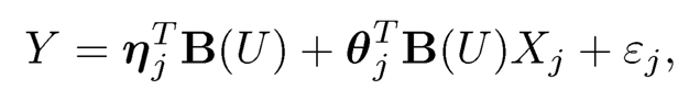
8.4.2 Varying coefficient models
Varying coefficient models are another class of popular nonparametric regression models in the literature and defined by
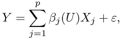 |
(8.19) |
where βj(U)’s are coefficient functions, depending on the observed (exposure) variable U such as age. An intercept can be included by setting X1 ≡1. Fan, Ma and Dai (2014) extended the NIS introduced in the last section to varying coefficient models, and Song, Yi and Zou (2014) further explored this methodology to the longitudinal data. From a different perspective, Liu, Li and Wu (2014) proposed a conditional correlation screening procedure based on the kernel regression approach.
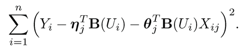
Fan, Ma and Dai (2014) started from the marginal regression problem for each Xi, j =1,..., p, i.e., finding aj(u) and bj(u) to minimize E{ (Y—aj(U)— bj(U)Xj)2|U = u}. Thus, the marginal contribution of Xj for predicting Y can be described as
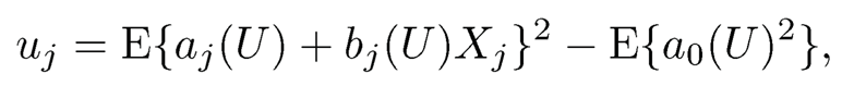
where a0(U) — E(Y|U).
Suppose that {(Ui, Xi, Yi), i = 1, ..., n} is a random sample from (8.19). Similar to the B-spine regression, we may obtain an estimate of aj(u), bj(u) and a0(u) through the basis expansion. Specifically, we fit the marginal model, using variables U and Xj,
where B (u) = {B1(u), . . ., Bdn(U)}T consists of normalized B-spline bases and ηj and θ are the coefficients for the functions aj(·) and bj(·), respectively. This leads to the following least-squares: find ηj and θj to minimize
This least-squares problem admits an analytic solution. Let
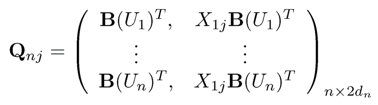
and Y = (Y1,⋯, Yn)T. Then,
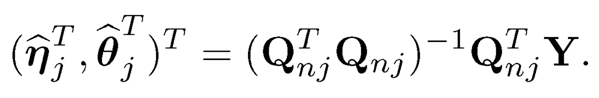
Thus the marginal coefficient functions aj(.) and bj(·) can be estimated as

We can estimate a0({) similarly (though this baseline function is not used in comparison of marginal utility).
The sample marginal utility for screening is
 |
(8.20) |
where ||·||2n is the sample average, defined in the same fashion as in the last section. The selected model is then M̂τ = {1 ≤ j ≤ p : ûnj ≥ τn} for the pre-specified data-driven threshold τn. Note that the baseline estimator ||â0(u)||2n is not needed for ranking the marginal utility.
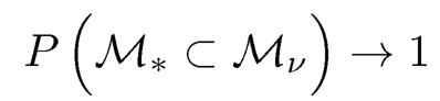
Fan, Ma and Dai (2014) established the sure screening property P(M, ⊂ Mτ) → for p = o(exp{n1-4κdn-3}) with κ > 0 under the regularization conditions listed in the previous section with an additional bounded constraint imposed on U, and assuming both Xj and E(Y|X, U), as well as the random error E follow distributions with the sub-exponential tails. Furthermore, the iterative screening and greedy iterative screening can be conducted in a manner similar to INIS.
Song, Yi and Zou (2014) proposed a feature screening procedure for varying coefficient models (8.19) under the setting of longitudinal data {(Uil, Yil, Xil) = 1, . . ., n l=1, …, ni}, where Xil = (Xi1, … Xilp)T. Instead of using Uj for the marginal utility, they proposed the following marginal utility:
 |
(8.21) |
where U is the bounded support of the covariate U, covariate U, and bj(u) is the minimizer of the marginal objective function Qj=E{Y-Xjbj(u)}2. To estimate Ωj, the predictor-specific B-spline basis Bj(u) ={Bj1(u),…,Bjdj(u)T is used, thus b̂nj= B(u)Tγ̂j, where γ̂j=(γ̂j1…,γjdj)T is the minimized of the sample objective function where U is the bounded support of the covariate U, and bj(u) is the minimizer of the marginal objective function Qj =E{Y — Xjbj (u)}2. To estimate Ωj, the predictor-specific B-spline basis Bj(u) ={Bj1(u),…,Bjdj(u)}T is used, thus b̂nj, =Bj(u)Tγ̂̂̂j, where γ̂j =(γ̂j1, …γ̂jdj)T is the minimizer of the sample
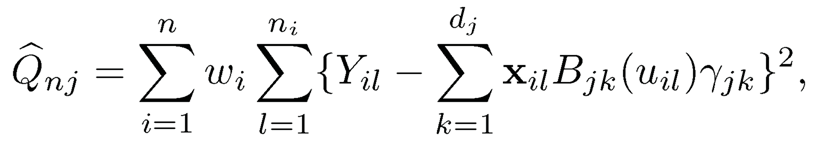
with the weight wi = 1 or 1/ni. Specifically,
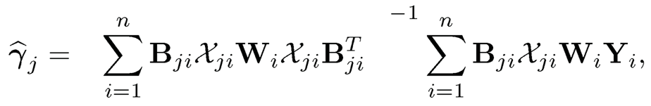
where Xji=diag (Xi1j, …, Xinij)ni×ni, Wi=diag (wi, …,wi)ni×ni,
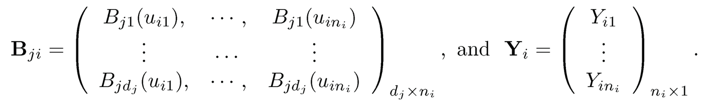
Therefore, a natural estimate of Ωj is
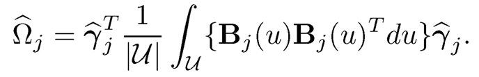 |
(8.22) |
The integral in (8.22) does not depend on data, and can be easily evaluated by numerical integration since u is univariate. As a result, we select the submodel with a pre-specified cutoff κn: Mκ ={1 ≤j ≤p : Ωi≥ κn}. Song, Yi and Zou (2014) also established the sure screening property of their procedure under the ultrahigh dimension setting with a set of regularity conditions.
From a different point of view, Liu, Li and Wu (2014) proposed another sure independent screening procedure for the ultrahigh dimensional varying coefficient model (8.19) based on conditional correlation learning (CC-SIS). Since (8.19) is indeed a linear model when conditioning on U, the conditional correlation between each predictor Xj and Y given U is defined similarly as the Pearson correlation:
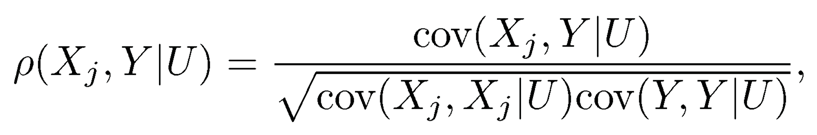
where cov(Xj, Y|U) =E(XjY|U)—E(Xj|U) E(Y|U) and the population level marginal utility to evaluate the importance of Xj is ρ*j0= E{ρ2(Xj, Y|U)}. To estimate ρ*j0, or equivalently, the conditional means E(Y|U), E(Y2|U), E(Xi|U), E(X2i|U) and E(XjY|U), with sample {(Ui,Xi,Yi), i = 1,...,n}, the kernel regression is adopted, for instance,

where Kh(t) = h-1K(t/h) is a rescaled kernel function. Therefore, all the plug-in estimates for the conditional means and conditional correlations ρ̂2(Xj, Y|Ui)’s are obtained, and thus also that of ρ*j0:
 |
(8.23) |
And the screened model is defined as

where the size d = [n4/5/ log(n4/5)] follows the hard threshold by Fan and Lv (2008) but modified for the nonparametric regression, where [a] is the integer part of a.
The sure screening property of CC-SIS has been established under some regularity conditions: (c1) the density function of u has continuous second-order derivative; (c2) the kernel function K(·) is bounded uniformly over its finite support; (c3) XjY, Y2, X2j satisfy the sub-exponential tail probability uniformly; (c4) all the conditional means, along with their first- and second-order derivatives are finite and the conditional variances are bounded away from 0. See Liu, Li and Wu (2014) for details.
8.4.3 Heterogeneous nonparametric models
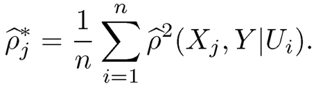
As is known, nonparametric quantile regression is useful to analyze the heterogeneous data, by separately studying different conditional quantiles of the response given the predictors. As to the ultrahigh-dimensional data, He, Wang and Hong (2013) proposed an adaptive nonparametric screening approach based on this quantile regression methodology.
At any quantile τ ∈ (0, 1), the true sparse model is defined as

where Qτ (Y |X) is the τth conditional quantile of Y given X = (X1,…, Xp)T. Thus, their population screening criteria can be defined as
 |
(8.24) |
with Qτ(Y|Xj), the Tth conditional quantile of Y given Xj, and Qτ(Y), the unconditioned quantile of Y. Thus Y and X are independent if and only if gτj= 0 for every τ ∈ (0, 1). Notice that

where ρτ(z) = z[r — I(z < 0)], the check loss function defined in Section 6.1.
To estimate gτj based on the sample {(Xi, Yi), i= 1,…, n}, one may consider the B-spline approximation based on a set of basis functions B(x) {B1(x), …, B dn(x)T. That is, one considers Q̂τ(Y|x) = B(x)TΓ̄j, where
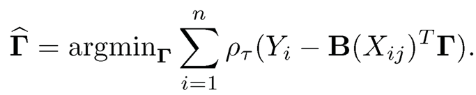
Furthermore, Qτ(Y) in (8.24) might be estimated by F-1Y,n (τ), the τth sample quantile function based on Y1,…, Yn. Therefore, gτi is estimated by
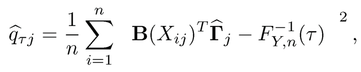 |
(8.25) |
and the selected submodel M̂γ= {1 ≤ j ≤ p: q̂τj ≥ γn} for some γn > 0.
To guarantee the sure screening property and control the false selection rate, the rth derivative of Qτ(YIXj) is required to satisfy the Lipschitz condition of order c, where r + c > 0.5; the active predictors need to have strong enough marginal signals; the conditional density function of Y given X is locally bounded away from 0 and infinity — this relaxes the sub-exponential tail probability condition in literature; however, global upper and lower bounds are needed for the marginal density functions of Xj‘s; and an additional restriction on cin, the number of basis functions is applied.
8.5 Model-free Feature Screening
Feature screening procedures described in Sections 8.1-8.4 were developed for a class of specific models. In high-dimensional modeling, it may be very challenging in specifying the model structure on the regression function without priori information. Zhu, Li, Li and Zhu (2011) advocated model-free feature screening procedures for ultrahigh dimensional data. We introduce several feature screening procedures without imposing a specific model structure on regression function in this section.
8.5.1 Sure independent ranking screening procedure
Let Y be the response variable with support ψy. Here Y can be both univariate and multivariate. Let X = (X1,…, XP)T be a covariate vector. Zhu, Li, Li and Zhu (2011) developed the notion of active predictors and inactive predictors without specifying a regression model. Consider the conditional distribution function of Y given X, denoted by F(y |X) =P(Y < y |X). Define the true model

If k ∈ M*, Xk is referred to as an active predictor, otherwise it is referred to as an inactive predictor. Again |M*|= s. Let XM*, an s x 1 vector, consist of all Xk with k ∈ M*. Similarly, let X,Mc*, a (p — s) x 1 vector, consist of all inactive predictors Xk with k ∈ MC*.
Zhu, Li, Li and Zhu (2011) considered a general model framework under which a unified screening approach was developed. Specifically, they considered that F(y X) depends on X only through BT XM for some p1 x K constant matrix B. In other words, assume that
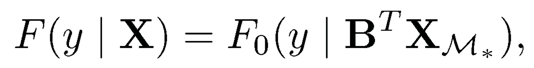 |
(8.26) |
where F0(· BTXM*) is an unknown distribution function for a given BTXM*. The model parameter B may not be identifiable. However, the identifiability of B is of no concern here because our primary goal is to identify active variables rather than to estimate B itself. Moreover, the model-free screening procedure does not require an explicit estimation of B.
Many existing models with either continuous or discrete response are special examples of (8.26). Moreover, K is as small as just one, two or three in frequently encountered examples. For instance, many existing regression models can be written in the following form:
 |
(8.27) |
for a continuous and
 |
(8.28) |
for a binary or count response by extending the framework of the generalized linear model to semiparametric regression, where h(·) is a monotonic function, g(·) is a link function, f2(·) is a nonnegative function, β1, β2 and β3 are unknown coefficients, and it is assumed that E is independent of X. Here h(·), g(·), f1(·) and f2(·) may be either known or unknown. Clearly, model (8.27) is a special case of (8.26) if B is chosen to be a basis of the column space spanned by β1, β2 and β3 for model (8.27) and by β1 and β2 for model (8.28). Meanwhile, it is seen that model (8.27) with h(Y) = Y includes the following special cases: the linear regression model, the partially linear model (Härdle, Liang and Gao, 2000) and the single-index model (Härdle, Hall and Ichimura, 1993), and the generalized partially linear single-index model (Carroll, Fan, Gijbels and Wand, 1997) is a special of model (8.28). Model (8.27) also includes the transformation regression model for a general transformation h(Y). As a consequence, a feature screening approach developed under (8.26) offers a unified approach that works for a wide range of existing models.
As before, assume that E(Xk) = 0 and Var(Xk) = 1 for k = 1,… ,p. By the law of iterated expectations, it follows that

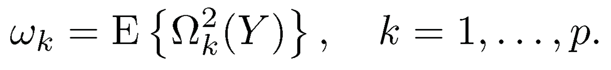
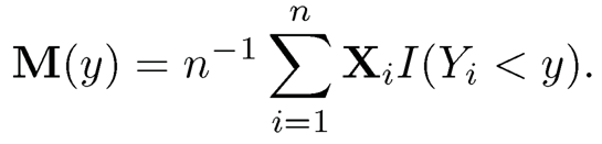
To avoid specifying a structure for regression function, Zhu, et al.(2011) considered the correlation between Xj and 1(Y < y) to measure the importance of the j-th predictor instead of the correlation between Xj and Y. Specifically, define M(y) = E{XF(y |X)}, and let Ωk(y) be the k-th element of M(y). Zhu, et al. (2011) proposed to use
 |
(8.29) |
as the marginal utility for feature screening. Intuitively, if Xk and Y are independent, Ωk(y) = 0 for any y ∈ ψy and ωk= 0. On the other hand, if Xk and Y are related, then there exists some y ∈ ψy such that Ωk(y) #0, and hence ωk must be positive. This is the motivation to employ the sample estimate of wk to rank all the predictors.
Suppose that {(Xi, Yi), i=1,⋯, n} is a random sample from {X, Y}. For ease of presentation, we assume that the sample predictors are all marginally standardized. For any given y, the sample moment estimator of M(y) is
Consequently, a natural estimator for ωk is
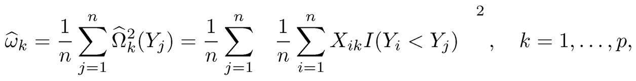
where Ω̂k (y) denotes the k-th element of M̂(y), and Xik denotes the k-th element of Xi Zhu, et al., (2011) proposed ranking all the candidate predictors Xk, k = 1, …,p, according to ω̂k from the largest to smallest, and then selecing the top ones as the acvive predictors.
Motivated by the following fact, Zhu, et al. (2011) established the consistency in ranking property for their procedure. If K = 1 and X ~ Np(0, σ2Ip) with unknown σ2 in model it follows a direct calculation that

where c(y) = |b|-1 ∫∞-∞vF0 (y |v ||b||)ø(v; 0, σ2) dv with ø(v; 0, σ2) being the density function of N(0, σ-2) at v. Thus, if E{c2(Y)} >0, then
 |
(8.30) |
and σk= 0 if and only if k ∈ M. This implies that the quantity ωk may be used for feature screening in this setting. Under much more general conditions than the normality assumption, Zhu, et al. (2011) showed that (8.30) holds. The authors further established a concentration inequality for ω̂k and, maxk∈Mc ω̂k < mink∈M* ω̂k, which is referred to as the property of consistency in ranking (CIR). Due to this property, they referred to their procedure as the sure independent ranking screening (SIRS) procedure. They studied several issues related to implementation of the SIRS method. Since the SIRS possesses the CIR property, the authors further developed a soft cutoff value for c—o3‘s to determine which indices should be included in M̂* by extending the idea of introducing auxiliary variables for thresholding proposed by Luo, Stefanski and Boos (2006). Zhu, et al. (2011) empirically demonstrated that the combination of the soft cutoff and hard cutoff by setting d = [n/ log(n)] works quite well in their simulation studies. Lin, Sun and Zhu (2013) proposed an improved version of the SIRS procedure for a setting in which the relationship between the response and an individual predictor is symmetric.
8.5.2 Feature screening via distance correlation
The SIRS procedure was proposed for multi-index models that include many commonly-used models in order to be a model-free screening procedure. Another strategy to achieve the model-free quality is to employ the measure of independence to efficiently detect linearity and nonlinearity between predictors and the response variable, and construct feature screening procedures for ultrahigh dimensional data. Li, Zhong and Zhu (2012) proposed a SIS procedure based on the distance correlation (Székely, Rizzo and Bakirov, 2007). Unlike the Pearson correlation coefficient, rank correlation coefficient and generalized correlation coefficient, which all are defined for two random variables, the distance covariance is defined for two random vectors which are allowed to have different dimensions.
The distance correlation between two random vectors U ∈ Rq1 and V ∈ Rq2 is defined by
 |
(8.31) |
where øU(t) and øv(s) are the marginal characteristic functions of U and V, respectively, øU,v(t,s) is the joint characteristic function of U and V, and
with Cd = π(1+d)/2/Γ{(1+ d)/2} (This choice is to facilitate the calculation of the integral). Here ||ø||2 = øø for a complex-valued function ø with ø being the conjugate of ø. From the definition (8.31), dcov2 (U, V) = 0 if and only if U and V are independent. Székely, Rizzo and Bakirov (2007) proved that

where

and (̂Ũ, Ṽ) is an independent copy of (U, V). Thus, the distance covariance between U and V can be estimated by substituting in its sample counterpart. Specifically, the distance covariance between U and V is estimated by
with

based on a random sample = 1, • • •, n} from the population (U, V)
Accordingly, the distance correlation between U and V is defined by

and estimated by plugging in the corresponding estimate of distance covariances. As mentioned above, dcov2 (U, V) = 0 if and only if U and V are independent. Furthermore, dcorr(U, V) is strictly increasing in the absolute value of the Pearson correlation between two univariate normal random variables U and V.
Let Y = (Y1,⋯, Yq)T be the response vector and X = (X1,…, Xp)T be the predictor vector. Motivated by the appealing properties of distance correlation, Li, et al. (2012) proposed a SIS procedure to rank the importance of the kth predictor Xk for the response using its distance correlation ω̂j = dcorr̂ (Xj, Y). Then, a set of important predictors with large ω̂ jis selected and denoted by M̂ ={j : ω̂ j ≥cn-k, for 1 ≤ j < ≤ p}.
Suppose that both X and Y satisfy the sub-exponential tail probability uniformly in p. That is, supp
 and E{exp(sYTY)} < ∞, for s > 0. Li, et al. (2012) proved that ω̂j is consistent to ωj uniformly in p,
 |
(8.32) |
for any 0 < γ < 1/2 — κ, some constants c1 > 0 and c2 > 0. If the minimum distance correlation of active predictors is further assumed to satisfy minj∈M* ωj ≥ 2cn-k, for some constants c> 0 and 0 <t < 1/2, as n →∞,
 |
(8.33) |
where s is the size of M*, the indices set of the active predictors is defined by
M*={1≤j≤p:F(Y|X) functionally depends on Xj for some Y ∈ ψy},
without specifying a regression model. The result in (8.32) shows that the feature screening procedure enjoys the sure screening property without assuming any regression function of Y on X, and therefore it has been referred to as distance correlation based SIS (DC-SIS for short). Clearly, the DC-SIS provides a unified alternative to existing model-based sure screening procedures. If (U, V) follows a bivariate normal distribution, then dcorr(U, V) is a strictly monotone increasing function of the Pearson correlation between U and V. Thus, the DC-SIS is asymptotically equivalent to the SIS proposed in Fan and Lv (2008) for normal linear models. The DC-SIS is model-free since it does not impose a specific model structure on the relationship between the response and the predictors. From the definition of the distance correlation, the DC-SIS can be directly employed for screening grouped variables, and it can be directly utilized for ultrahigh dimensional data with multivariate responses. Feature screening for multivariate responses and/or grouped predictors is of great interest in pathway analysis (Chen, Paul, Prentice and Wang, 2011).
As discussed in Section 8.1.3, there exist some predictors that are marginally uncorrelated with or independent of, but jointly are not independent of the response. Similar to marginal screening procedures introduced in Sections 8.1 and 8.2, the SIRS and DC-SIS both will fail to select such predictors. Thus, an iterative screening procedure may be considered, since both SIRS and DC-SIS do not rely on the regression function (i.e., the conditional mean of the response given the predictor). Thus, the iterative procedure introduced in Section 8.3 cannot be applied for SIRS and the DC-SIS because it may be difficult to obtain the residuals. Motivated by the idea of partial residuals, one may apply the SIRS and DC-SIS to the residual of the predictors on the selected predictor and the response. This strategy was used to construct an iterative procedure for the SIRS by Zhu, et al. (2011). Zhong and Zhu (2015) applied this strategy to the DC-SIS and developed a general iterative procedure for the DC-SIS, which consists of the three following steps.
T1. Apply the DC-SIS for Y and X and select p1 predictors, which are denoted by XM1 ={X(1)1, …, X(1)p1 }, where p1 < d, where d is a user-specified model size (for example, d = [n/ log n]). Let M = M1.
T2. Denote by X1 and Xc1 the corresponding design matrix of variables in M̂ and M̂c, respectively. Define Xnew= {In — X1 (XT1X1)-1 XT1}Xc1. Apply the DC-SIS for Y and Xnew and select p2 predictors XM2 {X(2)1 …, {X(2)p2. Update M̂ = M̂ U M2.
T3. Repeat Step T2 until the total number of selected predictors reaches d. The final model we select is M̂.
8.5.3 Feature screening for high-dimensional categorial data
Analysis of high-dimensional categorical data is common in scientific researches. For example, it is of interest to identify which genes are associated with a certain types of tumors. The types of tumors are categorical and may be binary if researchers are concerned with only case and control. This is a typical example of categorical responses. Genetic markers such as SNPs are categorical covariates. Classification and discriminant analysis are useful for analysis of categorical response data. Traditional methods of classification and discriminant analysis may break down when the dimensionality is extremely large. Even when the covariance matrix is known, Bickel and Levina (2004) showed that the Fisher discriminant analysis performs poorly in a minimax sense due to the diverging spectra. Fan and Fan (2008) demonstrated further that almost all linear discriminants can perform as poorly as random guessing. To this end, it is important to choose a subset of important features for high dimensional classification and discriminant analysis. High-dimensional classification is discussed in Chapter 12 in detail. This section introduces feature screening procedures for ultrahigh dimensional categorical data.
Let Y be a categorical response with K classes {Y1, Y2, …YK }. If an individual covariate Xj is associated with the response Y, then μjk = E(Xj|Y yk) are likely different from the population mean μj= E(Xj). Thus, it is intuitive to use the test statistic for the multi-sample mean problem as a marginal utility for feature screening. Based on this idea, Tibshirani, Hastie, Narasimhan and Chu (2002) propose a nearest shrunken centroid approach to cancer class prediction from gene expression data. Fan and Fan (2008) proposed using the two-sample t-statistic as a marginal utility for feature screening in high-dimensional binary classification. The authors further showed that the t-statistic does not miss any of the important features with probability one under some technical conditions.
Although variable screening based on the two-sample t-statistic (Fan and Fan, 2008) performs generally well in the high dimensional classification problems, it may break down for heavy-tailed distributions or data with outliers, and it is not model-free. To overcome these drawbacks, Mai and Zou (2013) proposed a new feature screening method for binary classification based on the Kolmogorov-Smirnov statistic. For ease of notation, relabel Y = +1, —1 to be the class label. Let F1j(x) and F2j(x) denote the conditional cumulative distribution function of Xj given Y = +1, —1, respectively. Thus, if Xj and Y are independent, then F1j(x) ≡ F2j(x). Based on this observation, the nonparametric test of independence may be used to construct a marginal utility for feature screening. Mai and Zou (2013) proposed the following Kolmogorov-Smirnov statistic to be a marginal utility for feature screening;
 |
(8.34) |
which can be estimated by ωnj= supx∈ℝ |F̂1j(x) - F̂2j (x)|, where |F̂1j(x) and F̂2j(x) are the corresponding empirical conditional cumulative distribution functions. Mai and Zou (2013) named this feature screening method as the Kolmogorov filter which sets the selected subset as
 |
(8.35) |
Under the conditions that  dn, Mai and Zou (2013) showed that the sure screening property of the Kolmogorov filter holds with probability approaching one. That is, P (M*⊆ M̂) →1 as n →∞.
The Kolmogorov filter is model-free and robust to heavy-tailed distributions of predictors and the presence of potential outliers. However, it is limited to binary classification. Mai and Zou (2015) further developed the fused Kol- mogorov filter for model-free feature screening with multicategory response, continuous response and counts response.
Cui, Li and Zhong (2014) proposed a sure independence screening using the mean-variance index for ultrahigh dimensional discriminant analysis. It not only retains the advantages of the Kolmogorov filter, but also allows the categorical response to have a diverging number of classes in the order of O(nκ) with some κ> 0.
To emphasize the number of classes being allowed to diverge as the sample size n grows, we use Kn for K. Denote by Fj(x) = P(Xj ≤ x) the unconditional distribution function of the jth feature Xj and Fjk(x) = P(Xj≤ yk) the conditional distribution function of Xj given Y =yk. If Xj and Y are statistically independent, then Fjk(x) = Fj(x) for any k and x. This motivates one to consider the following marginal utility
 |
(8.36) |
This index is named as the mean variance index of Xj given Y. Cui, Li and Zhong (2014) showed that

which is a weighted average of Cramér-von Mises distances between the conditional distribution function of Xj given Y =yk and the unconditional distribution function of Xj, where pk = P(Y = k). The authors further showed that MV(Xj|Y) = 0 if and only if Xj and Y are statistically independent. Thus, the proposal of Cui, Li and Zhong (2014) is basically to employ a test of the independence statistic as a marginal utility of feature screening for ultrahigh-dimensional categorical data.
Let {(Xij, Yi) : 1 ≤ i≤n} be a random sample of size n from the population (Xj, Y). Then, MV(Xj|Y) can be estimated by its sample counterpart
 |
(8.37) |
where p̂k = n-1, Σni=1 I(Yi=yk}, F̂jk(x)=n-1Σni=1 I{Xij≤x,Yi=yk}p̂k, and F̂j(x) n-1 Σni=1 I(Xij≤x}.
Without specifying any classification model, Cui, Li and Zhong (2014) defined the important feature subset by
 |
(8.38) |
MV(Xj|Y) is used to rank the importance of all features and the subset M = {j : MV̂(Xj|Y) ≥ cn-τ, for 1 ≤ j ≤ p} is selected. This procedure is referred to as the MV-based sure independence screening (MV-SIS). Assume that (1) for some positive constants c1 and c2,

and Kn = O(nκ) for κ ≥ 0; (2) for some positive constants c > 0 and 0 ≤  . Under Conditions (1) and (2), Cui, Li and Zhong (2014) proved that
where b is a positive constant and s =|M*|. As n →∞, P(M*⊆M̂)→1 for the NP-dimensionality problem logp = O(nα), where α < 1 — 2τ —κ with 0 ≤ τ < 1/2 and 0 ≤ κ< 1 — 2τ. Thus, the sure screening property of the MV-SIS holds.
It is worth pointing out that the MV-SIS is directly applicable for the setting in which the response is continuous, but the feature variables are categorical (e.g., the covariates are SNP). To implement the MV-SIS, one can simply use MV(Y|Xj) as the marginal utility for feature screening. When both response and feature variables are categorical, it is not difficult to use a test of independence statistic as marginal utility for feature screening. Huang, Li and Wang (2014) employed the Pearson χ2-test statistic for independence as a marginal utility for feature screening. They further established the sure screening procedure of their screening procedure under mild conditions.
8.6 Screening and Selection
In previous sections, we focus on marginal screening procedures, which enjoy the sure screening property under certain conditions. Comparing with variable selection procedures introduced in Chapters 3 - 6, the marginal screening procedures can be implemented with very low computational cost. To perform well, they typically require quite strong conditions. For instance, these marginal screening procedures may fail in the presence of highly correlated covariates or marginally independent but jointly dependent covariates. See Fan and Lv (2008) for detailed discussions on these issues. Although iterative SIS or its similar strategy may provide a remedy in such situations, it would be more natural to consider joint screening procedures that require screening and selection.
8.6.1 Feature screening via forward regression
Wang (2009) proposed using the classical forward regression method, which recruits one best variable at a time, for feature screening in the linear regression model (8.1). Given a subset S that is already recruited, the next step is to find one variable Xĵ so that (Xs Xĵ} has the smallest RSS among all models {(Xs, Xj), j ∈ S}. Specifically, starting with the initial set S(0) = Ø, and for k =1,⋯,n, let ak ∈S(k-1)c, the complement of S(k-1), be the index so that the covariate Xak along with all predictors in S(k-1) achieves the minimum of the residual sum of squares over j ∈ S(k-1)c, and set S(k)=S(k-1) ∪ { ak}accordingly. Wang (2009) further suggested using the extended BIC (Chen and Chen, 2008) to determine the size of the active predictor set. The extended BIC score for a model M is defined as

where ∂-2M is the mean squared error under model M, and |M| stands for the model size of model M. Choose

and set Ŝ= S(m̂). Wang (2009) imposed the following conditions to establish the sure screening property. Recall M* = {j : βj #0}, the index set of active predictors, defined in Section 8.1.1.
(B1) Assume that both X and ε in model (8.1) follow normal distributions.
(B2) There exist two positive constants 0 < τmin < τmax < ∞ such that τrain < λmin (Σ) < τmax(Σ) < τmax, where Σ = E(XXT).
(B3) Assume that ||β||2≤ Cβ for somem constant Cβ and min1≤j≤p|βj|≥ vβn-ξmin for some positive constants vβ and γmin > 0. ||β||2 ≤ Cβ for some constant Cβ and min1<j≤|β| ≤
(B4) There exists constants and v such that log(p) ≤vnξ, |M*| ≤ vnξ0, and ξ+6ξ0+12ξmin<1.
Theorem 8.4 Under model (8.1) and Conditions (B1)-(B-4), it follows that

8.6.2 Sparse maximum likelihood estimate
Suppose that a random sample was collected from an ultrahigh dimensional generalized linear model with the canonical link, and the log-likelihood function is
 |
(8.39) |
In genetic study, we may encounter such a situation in which we have resources to examine only k genetic markers out of a huge number of potential genetic markers. Thus, it requires the feature screening stage to choose k covariates from p potential covariates, in which k ≪ p. Xu and Chen (2014) formulates this problem as maximum likelihood estimation with l0 constraint. They define the sparse maximum likelihood estimate (SMLE) of β to be
 |
(8.40) |
where ||·|| denotes the l0-norm. This problem of finding the best subset of size k finds its applications also in guarding the spurious correlation in statistical machine learning (Fan and Zhou, 2016; Fan, Shao, and Zhou, 2018) who also independently used the following algorithm (Section 2.3, Fan and Zhou, 2016).
Let M̂ = {1 ≤ j ≤ p:-β̂[k]j #0} correspond to nonzero entries of β̂[k]. For a given number k, the SMLE method can be considered as a joint-likelihood-supported feature screening procedure. Of course, the maximization problem in (8.40) cannot be solved when p is large. To tackle the computation issue, Xu and Chen (2014) suggested a quadratic approximation to the log-likelihood function. Let Sn(β) = ln(β) be the score function. For a given β, approximate ln(γ) by the following isotropic quadratic function
 |
(8.41) |
for some scaling parameter u > 0. The first two terms in (8.41) come from the first-order Taylor’s expansion of ln(β), while the third term is viewed as an l2-penalty to avoid -γ too far away from β. The approximation (8.41) coincides with (3.77) in the iterative shrinkage-thresholding algorithm introduced in Section 3.5.7 Instead of maximizing (8.40) directly, we iteratively update β(t) by
for a given β(t) in the t-th step. Due to the form of hn(-γ; β), the solution β(t+1) is a hard thresholding rule and has an explicit form. Let

and rk be the kth largest value of {g|, ⋯,|gp|}. Then

which is a hard-thresholding rule. Thus, Xu and Chen (2014) referred to this algorithm as the iterative hard thresholding (IHT) algorithm. Notice that

for any 0 with proper chosen u. These two properties make the IHT algorithm a specific case of the MM algorithm and lead to the ascent property of the IHT algorithm. That is, under some conditions, ln(β(t+1)) ≥ ln(β(t)) Therefore, one can start with an initial β(0) and carry out the above iteration until ||β(t+1) -β(t) ||2 falls below some tolerance level.
To see why SMLE can be used for feature screening, let us examine the case of the normal linear regression model, in which b’ (θ) = θ. Thus, for any β(t), g = (1 - u-1)β(t) +u-1YTY. As a result, if u = 1, gj is proportional to the sample correlation between Y and Xj. Clearly, the SMLE with u = 1 is a marginal screening procedure for normal linear models.
Xu and Chen (2014) further demonstrated that the SMLE procedure enjoys the sure screening property in Theorem 8.5 under the following conditions. Recall the notation M*= {1 ≤j ≤ p : βj #0} the true model, where β* (β*1, ⋯ β*p)T is the true value of β. For an index set S ⊂{1, ⋯, p}, {βj, j ∈ S} and β*s= {β*j, j ∈ S}.
(C1) log p = O(nα) for some 0 ≤ α< 1.
(C2) There exists w1, w2 > 0 and some nonnegative constants τ1, τ2 such that

(C3) There exist constants c1 > 0, δ1 > 0, such that for sufficiently large n, λmin{n-1 Hn(βS)} ≥c1 for βs ∈ {βS: ||βS-β*S||≤δ1} and S∈{M: M*⊂M; ||M||0 ≤2k}, where Hn(βS) is the Hessian matrix of ln(βM)
(C4) There exist positive constants c2 and c3, such that all covariates are bounded by c2, and when n is sufficiently large,
Theorem 8.5 Under model (8.39) and Conditions (C1)-(C4) with τ1+τ2 < (1 — α)/2, let M̂ be the model selected (8.40). It follows that
as n →∞.
8.6.3 Feature screening via partial correlation
Based on the partial correlation, Biihlmann, Kalisch and Maathuis (2010) proposed a variable selection method for the linear model (8.1) with normal response and predictors. To extend this method to the elliptical distribution, Li, Liu and Lou (2017) first studied the limiting distributions for the sample partial correlation under the elliptical distribution assumption, and further developed feature screening and variable selection for ultra-high dimensional linear models.
A p-dimensional random vector X is said to have an elliptical distribution if its characteristic function E exp(itT X) can be written as exp(itTμ)ø(tT Σt) for some characteristic generator ø(·). We write X ~ ECp(μ, Σ, ø). Fang, Kotz and Ng (1990) gives a comprehensive study on elliptical distribution theory. Many multivariate distributions such as multivariate normal distribution and multivariate t-distribution are special cases of elliptical distributions.
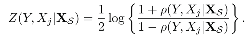
For an index set S ⊆ {1, 2, ⋯, p}, define XS = {Xj : j ∈ S} to be a subset of covariates with index set S. The partial correlation between two random variables Xj and Y given a set of controlling variables Xs, denoted by ρ(Y, Xj |Xs), is defined as the correlation between the residuals rxj, XS, and rY,XS from the linear regression of Xj on Xs and that of Y on XS, respectively.
The corresponding sample partial correlation between Y and Xj given XS is denoted ρ̂(Y, Xj| XS) . Suppose that (XT1, Y1), ⋯, (XTn, Yn) are a random samples from an elliptical distribution ECp+1(μ, Σ, ø) with all finite fourth moments and kurtosis K. For any j = 1, ⋯ p, and S ⊆ {j}c with cardinality |S|= o(√n), if there exists a positive constant δ0 such that λmin{cov(Xs)} > δ0, then
 |
(8.42) |
See Theorem 1 of Li, Liu and Lou (2017). Further apply the Fisher Z-transformation on ρ̂(Y, Xj|XS) and ρ(Y, Yj |XS)
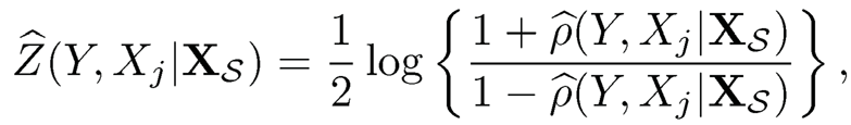 |
(8.43) |
 |
(8.44) |
Then, it follows by the delta method and (8.42) that
 |
(8.45) |
The asymptotic variance ρ̂(Y, Xj|XS) in (8.42) involves ρ(Y, Xj|XS), while the asymptotic variance of Ẑ(Y, Xj, |XS) does not. Thus, it is easier to derive the selection threshold for Ẑ(Y, Xj, |XS) than for ρ̂(Y, Xj, |XS)
Let 0 be the empty set, and ρ̂(Y, Xj, |Xø) and ρ(Y, Xj, |Xø) stand for ρ̂(Y, Xj) and ρ(Y, Xj), respectively. Then (8.42) is also valid for S = ø:
 |
(8.46) |
which was shown in Theorem 5.1.6 of Muirhead (1982).
The limiting distributions of partial correlation and sample correlation are given in (8.42) and (8.46), respectively. They provide insights into the impact of the normality assumption on the variable selection procedure proposed by Biilhmann, et al. (2010) through the marginal kurtosis under ellipticity assumption. This enables one to modify their algorithm by taking into account the marginal kurtosis to ensure its good performance.
To use partial correlation for variable selection, Biihlmann, Kalisch and Maathuis (2010) imposed the partial faithful condition which implies that
 |
(8.47) |
if the covariance matrix of X is positive definite. That is, Xj is important (or βj # 0) if and only if the partial correlations between Y and Xj given all subsets S contained in {j}c are not zero. Extending the PC-simple algorithm proposed by Biihlmann, Kalisch and Maathuis (2010), Li, Liu and Lou (2017) proposed to identify active predictors by iteratively testing the series of hypotheses

where m̂reach = min {m: |Â[m] ≤ m}, and |Â[m] is the chosen model index set in the mth step with cardinality |Â[m]|. Based on the limiting distribution (8.45), the rejection region at level a is |Ẑ(Y, Xj, |XS)| > √11+κzα+2/√n with κ̂ being a consistent estimate of K, where z, is the critical value of N(0, 1) at level α. In practice, the factor √n in the rejection region is replaced by √n — 1 — |S| due to the loss of degrees of freedom used in the calculation of residuals. Therefore, an equivalent form of the rejection region with small sample correction is
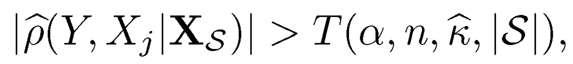 |
(8.48) |
where
 |
(8.49) |
with κ being estimated by its sample counterpart:
 |
(8.50) |
where Xj is the sample mean of the j-the element of X and Xij is the j-th element of Xi. In practice, the sample partial correlations can be computed recursively: for any k ∈ S,
 |
(8.51) |
A thresholded partial correlation variable selection can be summarized in the following algorithm, which was proposed by Li, Liu and Lou (2017).
Algorithm for TPC variable selection.
S1.Set m = 1 and S = Ø, obtain the marginally estimated active set by

S2.Based on Â[m-1], construct the mth step estimated active set by
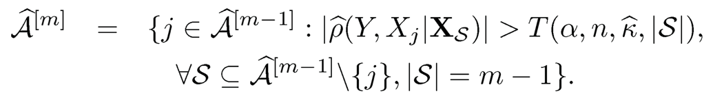
S3. S3. Repeat S2 until m = m̂reach
This algorithm results in a sequence of estimated active sets

Since κ = 0 for normal distributions, the TPC is indeed the PC-simple algorithm proposed by Biihlmann, et al. (2010) under the normality assumption. Thus, (8.45) clearly shows that the PC-simple algorithm tends to over-fit (under-fit) the models under those distributions where the kurtosis is larger (smaller) than the normal kurtosis 0. As suggested by Biihlmann, et al. (2010), one further applies the ordinary least squares approach to estimate the coefficients of predictors in |Â[mreach] chi after running the TPC variable selection algorithm.
Li, Liu and Lou (2017) imposed the following regularity conditions to establish the asymptotic theory of the TPC. These regularity conditions may not be the weakest ones.
(D1) The joint distribution of (XT, Y) satisfies the partial faithfulness condition (8.47).
(D2) (XT, Y) follows ECp+1(μ,, Σ, ø with Σ > 0. Furthermore, there exists s0 > 0, such that for all 0 < s < s0,

(D3) There exists δ > —1, such that the kurtosis satisfies κ> δ —1.
(D4) For some cn = O(n—d), 0 < d < 1/2, the partial correlations ρ(Y, Xj|Xs) satisfy inf |ρ(Y, Xj |XS)| :1 <j ≤ p, S ⊆ {j}c |S| ≤ d0, ρ(Y, Xj|Xs) #0} ≥cn.
(D5) The partial correlations ρ(Y, Xj|XS) and ρ(Xj, XklXS) satisfy:
i). sup { |ρ(Y, Xj|Xs)| :1 <j ≤ p, S ⊆ { j}c |S| ≤ d0} ≤τ <1,
ii). sup {|ρ(Xj, Xk |XS)}| : 1 ≤ j # k ≤ p, S ⊆ {j, k}c, |S|≤ d0} ≤ τ < 1.
The partial faithfulness condition in (D1) ensures the validity of the TPC method as a variable selection criterion. The assumption on elliptical distribution in (D2) is crucial when deriving the asymptotic distribution of the sample partial correlation. Condition (D3) puts a mild condition on the kurtosis, and is used to control Type I and II errors. The lower bound of the partial correlations in (D4) is used to control Type II errors for the tests. This condition has the same spirit as that of the penalty-based methods which requires the non-zero coefficients to be bounded away from O. The upper bound of partial correlations in the condition i) of (D5) is used to control Type I error, and the condition ii) of (D5) imposes a fixed upper bound on the population partial correlations between the covariates, which excludes the perfect collinearity between the covariates.
Based on the above regularity conditions, the following consistency property has been established. First we consider the model selection consistency of the final estimated active set by TPC. Since the TPC depends on the significance level a = an, we rewrite the final chosen model to be (an).
Theorem 8.6 Consider linear model (8.1). Under Conditions (D1)-(D5), there exists a sequence an → 0 and a positive constant C, such that if do is fixed, then for p = o(exp(nξ)), 0 < ξ< 1/5, the estimated active set can be identified with the following rate
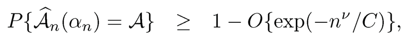 |
(8.52) |
where ξ< v < 1/5; and if d0= O(nb), 0 < b < 1/5, then for p = o(exp(nξ)), 0 <ξ < 1/5 — b, (8.52) still holds, with ξ < b<v < 1/5.
This theorem is due to Li, Liu and Lou (2017). Theorem 8.6 implies that the TPC method including the original PC-simple algorithm enjoys the model selection consistency property when dimensionality increases at an exponential rate of the sample size. Biffhmann, et al. (2010) suggested that αn= 2{1 — Ø(cn√n/ (1+ κ)/2)}.
Biihlmann, et al. (2010) established results in Theorem 8.6 for the normal linear model with pn increasing at a polynomial rate of n. In other words, Theorem 8.6 relaxes normality assumptions on model error and dimensionality from the polynomial rate to the exponential rate.
Since the first step in the TPC variable selection algorithm is indeed correlation learning, it is essentially equivalent to the SIS procedure described in Section 8.1.1. Thus, it is of interest to study under what conditions, the estimated active set from the first step of the TPC, denoted by Â[1]n (αn), possesses the sure screening property. To this end, we impose the following conditions on the population marginal correlations:
(D6) inf flp„(Y, X3)1 : j = 1,, p, p„(y, X3) 0} > c„, where 0(n—d), and 0 < d < 1/2.
(D7) sup { X3)1 : j = 1, ,p„,} < T <1.
Theorem 8.7 Consider linear model (8.1) and assume (D1)-(D3), (D6) and (D7). For p = 0(exp(nξ)), where 0 < ξ< 1, there exists a sequence an 0 such that P{Â[1]n A} ≥ 1-O{exp(-nv/C*)}, where C* is a positive constant and ξ< v < 1/5.
This theorem confirms the sure screening property of the marginal screening procedure based on the Pearson correlation under a different set of regularity conditions given in Section 8.1.1.
8.7 Refitted Cross-Validation
The impact of spurious correlation on residual variance estimation was demonstrated in Section 1.3.3 (see Figure 1.9 there). The refitted cross-validation (RCV) method was briefly introduced in Section 3.7 for estimating the error variance in ultrahigh dimensional linear regression. It is effective in reducing the impact of spurious correlated variables and hence a good companion with sure screening methods, where many variables can be spurious. As an effective tool to get rid of the effect of spurious correlated variables, the RCV method can be used in many regression models beyond linear models. This section provides additional insights.
8.7.1 RCV algorithm
Consider a general regression model
 |
(8.53) |
where E is a random error with E(ε| X) = 0 and Var(ε|X) =σ2. Of interest is to estimate σ2. In the presence of ultrahigh dimensional covariates, we typically assume that only a small number of covariates are active. In other words, m(x) depends on x only through a low dimensional subvector of x. Thus, model selection techniques are used to identify the small subset of active predictors. Due to ultra-high dimensionality, the selected model very likely includes some predictors that are spuriously correlated with the response. As a result, the mean squared errors of the selected model leads to an underestimate of σ2. Thus, the estimation of σ2 indeed is challenging.
The RCV method is to randomly split the entire sample into two data subsets, denoted by D1 and D2 respectively. We use D1 for model selection, and then refit the selected model to D2. This leads to an estimate of σ2, denoted by σ̂21. Intuitively, the selected model based on D1 may include some spuriously correlated predictors, which likely are not spuriously correlated predictors any more in D2 due to randomly splitting, and will play minor roles in estimating σ2 based on D2. Thus, σ̂21 may be a good estimate of o-2. Unlike the cross-validation method, both D1 and D2 play an important role, and their sample size cannot be too small since we need to ensure enough sample size in D1 to select a good model and ensure enough sample size in D2 to achieve estimation accuracy.
Similarly, we may use D2 for model selection, and then use D1 for error variance estimation. This leads to another estimate of σ2, denoted by σ̂22. Then the RCV estimate of σ2 is the average of σ̂21 and
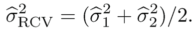 |
(8.54) |
Similar to (3.103), one may consider a weighted average of σ̂21 and σ̂21 as an estimate of σ2. Figure 8.3 depicts the algorithm for estimating o-2 by using the RCV method for general regression settings.
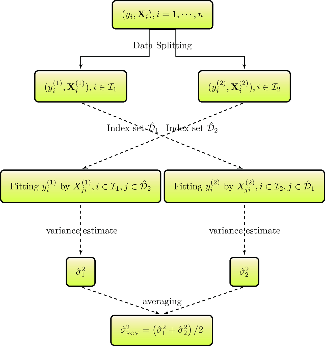
Figure 8.3: RCV algorithm for estimating σ2. Adapted from Chen, Fan and Li (2018).
8.7.2 RCV in linear models
Consider linear regression model
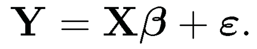
Let XM be the submatrix containing the columns of X that are indexed by M and denote PM =XM (XTM XM)-1XTM, the corresponding projection matrix of XM.
A naive two-stage procedure consists of (a) selecting a model M̂ by variable selection or feature screening procedures introduced in Chapter 3 and Sections 8.1-8.6 and (b) then estimate σ2 by the mean squared errors based on model
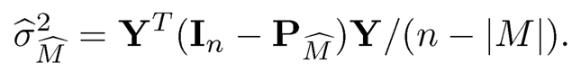
Denote γ̂2n =εTPM̂ ε/εTε. Thus, σ̂2M̂ can be rewritten as
Fan, Guo and Hao (2012) showed that under certain regularization conditions, σ̂̂2n /(1-γ̂̂2n) →σ2 in probability, and
 |
(8.55) |
in distribution. Thus, if γ̂̂2n does not tend to 0 in probability, the naive estimator σ̂2M̂ is not consistent. Fan, Guo and Hao (2012) further showed that under certain conditions and if log(p/n) = O(1), γ̂2n =OP{|M| log(p)/n}. This rate is often sharp. This implies that γ̂2n may may converge to a positive constant with a non-negligible probability and explains the reason why the naive estimator underestimates the noise level.
The RCV method for the linear model is to randomly split (X, Y) into two even data sets (X1, Y1) and (X2, Y2), based on which, we can obtain two selected models M̂1 and M̂2 by a variable selection such as the Lasso and the SCAD or a feature screening procedure such as SIS, respectively. Then we fit data subset (X2, Y2) to model M1 and calculate its mean squared errors a?, and fit data subset (X1, Y1) to model M̂2 to obtain its mean squared errors σ̂22. More specifically,
for k = 1 and 2, where P3-k is the projection matrix associated with model Mk based on data (X3-k, Y3-k). As defined in (8.54), σ̂2RCV is the average of σ̂21 and σ̂22. Fan, Guo and Hao (2012) studied the theoretical properties of σ̂2RCV in the following theorem.
Theorem 8.8 Suppose that (a) the errors εi, i= 1, ⋯, n are independent and identically distributed with zero mean and finite variance σ2 and independent of the design matrix X; and (b) there is a constant λ0 > 0 and bn such that bn/n → 0 such that P{Ømin(bn) ≥ λ0} = 1 for all n, where Ørnin(m) = minM:|M|≤m {λmin(n-1XTM XM)}. Further assume that E(ε41) < ∞ and with probability tending to one, the selected models M1 and M2 include the true model M ={j : βj #0} with max{|M1|, |M|2} ≤ bn. Then
 |
(8.56) |
in distribution.
Assumption (a) and the assumption on the finite fourth moment of ε are natural. Assumption (b) implies that the variables selected in Stage 1 are not highly correlated. In the presence of highly correlated predictors in the selected variables, ridge regression or penalization methods can be applied in the refitted stage. Moreover, robust regression techniques can be utilized in the refitted state in the of error distribution.
This theorem requires the model selection procedure used for obtaining M̂1 and M̂2 possesses a sure screening property rather than selection consistency. As shown in Theorem 8.1, the SIS procedure enjoys the sure screening property and can be used for fit and M̂1 and M̂1.
This theorem implies that under certain conditions, the RCV estimate σ̂2RCV and the oracle estimator σ̂2O =||ε||2 /n share the same asymptotic normal distribution. It is of interest to compare the RCV estimator with error variance estimators 6-2L, the mean squared errors of the Lasso estimate, and i’:”CAD, the mean squared errors of the SCAD estimate. Fan, Guo and Hao (2012) established the asymptotic normality of σ̂̂2L and σ̂̂2SCAD. Under extra strong assumptions in additions to the assumptions in Theorem 8.8, σ̂2L and σ̂2SCAD may have the asymptotic normal distribution in (8.55). Simulation results in Fan, et al. (2012) imply that the impacts of different variable selection and feature screening procedures such as SIS and Lasso on the performance of RCV are negligible. Both σ̂2L and σ̂2SCAD may lead to an underestimate.
As mentioned in Fan, Guo and Hao (2012), there are two natural extensions of the aforementioned RCV techniques.
The first natural extension is to use a K-fold data splitting technique rather than twofold splitting. That is, one can randomly split the data into K groups and select the model with all groups except one, which is used to estimate the variance with refitting. This may improve the sure screening probability with this K-fold method since more data are utilized in the first stage. However, there are only [n/ K] data points in the second stage for refitting. This means that the number of variables that are selected in the first stage should be much less than [n/K]. This makes the ability of sure screening difficult in the first stage. For this reason, the twofold RCV is recommended.
The second extension is to repeatedly and randomly split data. There are many ways to split the data randomly. Hence, many RCV variance estimators can be obtained. We may take the average of the resulting estimators. This reduces the influence of the randomness in the data splitting, while this may significantly increase the computational cost.
8.7.3 RCV in nonparametric regression
The idea of the RCV method is applicable for nonparametric and semi-parametric regression models. This section focuses on high dimensional additive models introduced in Section 8.4.1. Chen, Fan and Li (2018) found that the spurious correlation may be much more severe in ultrahigh dimensional nonparametric regression models than in the linear model.
Figure 8.4: Distributions of the maximum “linear” and “nonparametric” spurious correlations for s = 1 and s = 2 (left panel, n = 50 and p = 1000) and their consequences on the estimating of noise variances (right panel). The legend ‘LM’ stands for linear model, and ‘AM’ stands for additive model, i.e., a nonparametric model. Adapted from Chen, Fan and Li (2018).
To illustrate the spurious correlation in the nonparametric regression setting, we generate a random sample (XTi, Yi), i=1, ⋯, n = 50 from Np+1 (O, Ip+1). As in Section 1.3.3, we compute the maximum “linear” spurious correlation rL=max1≤j≤p |corr̂ (Xj, Y)| and the maximum “nonparametric” spurious correlation rN= max1≤j≤p Icorr̂ (f̂j (Xj), Y)|, where f̂j(Xj) is the best cubic spline fit of variable Xj to the response Y, using 3 equally spaced knots in the range of the variable Xj which create dn = 6 B-spline bases for Xj. The concept of the maximum spurious “linear” and spurious “nonpara-metric” (additive) correlations can easily be extended to s variables, which are the correlation between the response and fitted values using the best subset of s-variables. Based on 500 simulated data sets, Figure 8.4 depicts the results, which show the big increase of spurious correlations from linear to nonparametric fit. As a result, the noise variance is significantly underestimated.
Similar to Section 8.4.1, we can approximate mj(x) =Σdjk=1 γjkBjk(x), where Bjk(·),k =1 , ⋯ , dj is a set of B-spline bases with knots depending on j. For ease of notation and without loss of generality, assume that all dj's are the same and are denoted by dn. Replacing mj(Xj) by its spline approximation, we have
which can be viewed as an extended linear model. The strategy of the RCV method for linear models can be directly used for the ultrahigh dimensional additive model. Note that the dimension for this extended linear model is dnp.
A naive estimate σ̂2can be described as follows. We first apply a feature screening procedure such as NIS and DC-SIS to the whole data set, and fit the data to the corresponding selected spline regression model, denoted by D* the indices of all true predictors and D̂ the indices of the selected predictors respectively, satisfying the sure screening property D* ⊂ D̂. Then, we minimize
 |
(8.57) |
with respect to γ. Denote by γ̂jk the resulting least squares estimate. Then, the nonparametric residual variance estimator is
Here we have implicitly assumed that the choice of D and dn is such that n≥ |D̂|·dn. Let PD̂ be the corresponding projection matrix of model (8.57) with the entire samples, denoted by γ̂2n =εTPD̂ε/εTε. Under a certain regularity condition, Chen, Fan and Li (2018) show that (8.55) is still valid, and
 |
(8.58) |
These results imply that σ̂2D̂-- may significantly underestimates σ2 due to spurious correlation.
The RCV method is to randomly split the random samples into two even data subsets denoted by D1 and D2. We apply a feature screening procedure (e.g., DC-SIS or NIS) for each set, and obtain two index sets of selected x- variables, denoted by D̂1 and D̂2. Both of them retain all important predictors. The refitted cross-validation procedure consists of three steps. In the first step, we fit data in DI to the selected additive model D̂3-1 for l = 1 and 2 by the least squares method. These results in two least squares estimates γ̂(3-l) based on D1, respectively. In the second step, we calculate the mean squared errors for each fit:
for l = 1 and 2. As defined in (8.54), σ̂2RCV is the average of σ̂21 and σ̂22. Under certain regularity conditions, Chen, Fan and Li (2018) showed that the asymptotic normality of σ̂2RCV in (8.56) still holds.
8.8 An Illustration
This section is devoted to an illustration of the feature screening procedures and RCV method via an empirical analysis of a supermarket data set (Wang, 2009). This illustration is adapted from Chen, Fan and Li (2018). This supermarket data set consists of a total of n = 464 daily records of the number of customers (Yi) and the sale amounts of p = 6, 398 products, denoted as Xi1, ⋯, Xip, which are used as predictors. For data confidentiality, both the response and predictors are marginally standardized so that they have zero sample mean and unit sample variance. We consider an additive model

where εi is a random error with E(εi) = 0 and Var(εi Xi) = σ2.
Table 8.1: Error variance estimate for market data. Adapted from Chen, Fan and Li (2018)
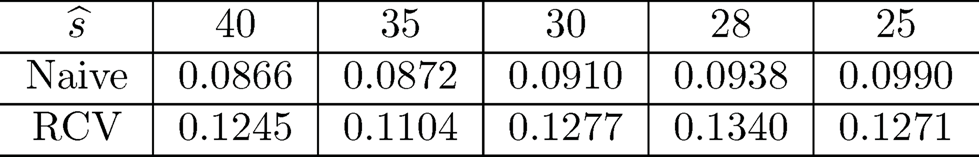
In this example, we use DS-SIS for feature screening in the model selection stage since it is a model-free feature screening procedure and possesses the sure screening property. To illustrate the impact of the selected model size ŝ on the error variance estimation, we let = 25, 30, 35 and 40. Since the sample size n = 464, the suggested threshold ŝ= [n4/5/ log(n4/5)] = 28 for nonparametric screening by Liu, Li and Wu (2014) is also considered. For these five model sizes, we obtain the naive error variance estimate and the RCV error variance estimate introduced in Section 8.7.3. Table 8.1 depicts the resulting error variance estimates. Table 8.1 clearly implies that the RCV estimate of error variance is stable with different choices of while the naive error variance estimate reduces as increases. With ŝ= 28, the naive error variance estimate equals 0.0938, while the RCV error variance estimate equals 0.1340, an 43% increase of the estimated value when the spurious correlation is reduced.
Regarding the selected models with ŝ= 28 predictors as a correct model and ignoring the approximation errors (if any) due to B-spline, we apply the Wald’s χ2-test for the hypothesis whether (γj1, ⋯γjdj)T, equals zero, namely whether the jth variable is active when the rest of the variables are included. The Wald’s χ2 statistics may provide us a rough picture of whether Xj is active or not. The Wald’s χ2-test with the naive error variance estimate concludes 12 significant predictors at significant level 0.05, while the Wald’s χ2-test with the RCV error variance estimate concludes seven significant predictors at the same significance level. Figure 8.5 depicts the Q-Q plot of values of the χ2- test statistic of those insignificant predictors identified by the Wald’s test.Figure 8.5 clearly shows that the χ2-test values using the naive error variance estimate systematically deviate from the 45-degree line. This implies that the naive method results in an underestimate of error variance, while the RCV method results in a good estimate of error variance.
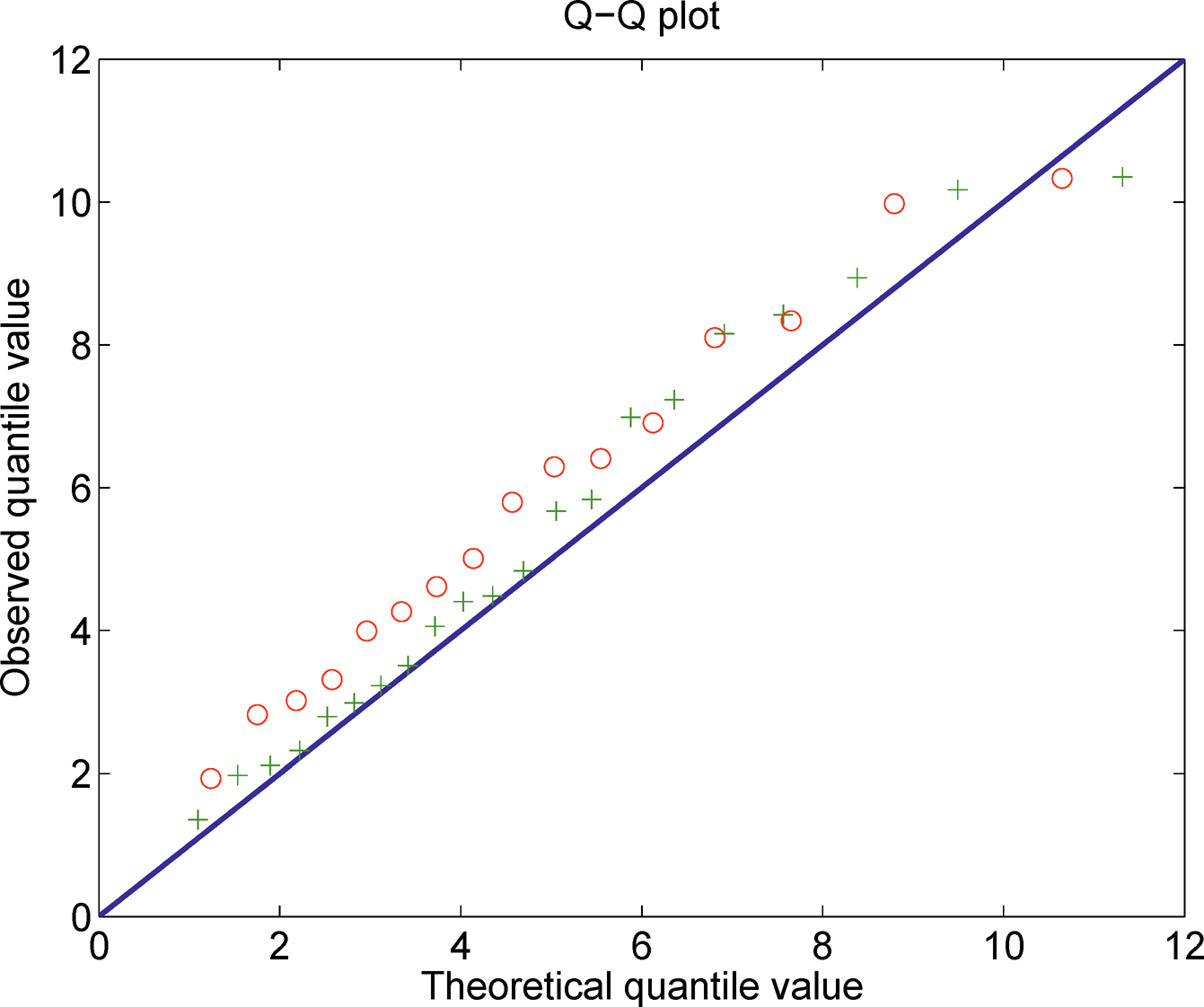
Figure 8.5: Quantile-quantile plot of the χ2-test values. “o” stands for χ2-test using the naive error variance estimate. “+” stands for χ2-test using the RCV error variance estimate. Taken from Chen, Fan and Li (2018).
The Wald’s test at level 0.05 affirms that seven predictors, X11, X139, X3, X39, X6, X62 and X42, are significant. We refit the data with the additive model with these 7 predictors. The corresponding mean squared errors is 0.1207, which is close to the σ̂2RCV = 0.1340. Note that σ2 is the minimum possible prediction error. It provides a benchmark for other methods to compare with and is achievable when modeling bias and estimation errors are negligible.
To see how the above selected variables perform in terms of prediction, we further use the leave-one-out cross-validation (CV) and five-fold CV to estimate the mean squared prediction errors (MSPE). The leave-one-out CV yields MSPE=0.1414, and the average of the MSPE obtained from five-fold CV based on 400 randomly splitting data yields is 0.1488 with the 2.5th percentile and 97.5th percentile being 0.1411 and 0.1626, respectively. The MSPE is slightly greater than σ̂2RCV. This is expected as the uncertainty of parameter estimation has not been accounted for. This bias can be corrected with the theory of linear regression analysis.
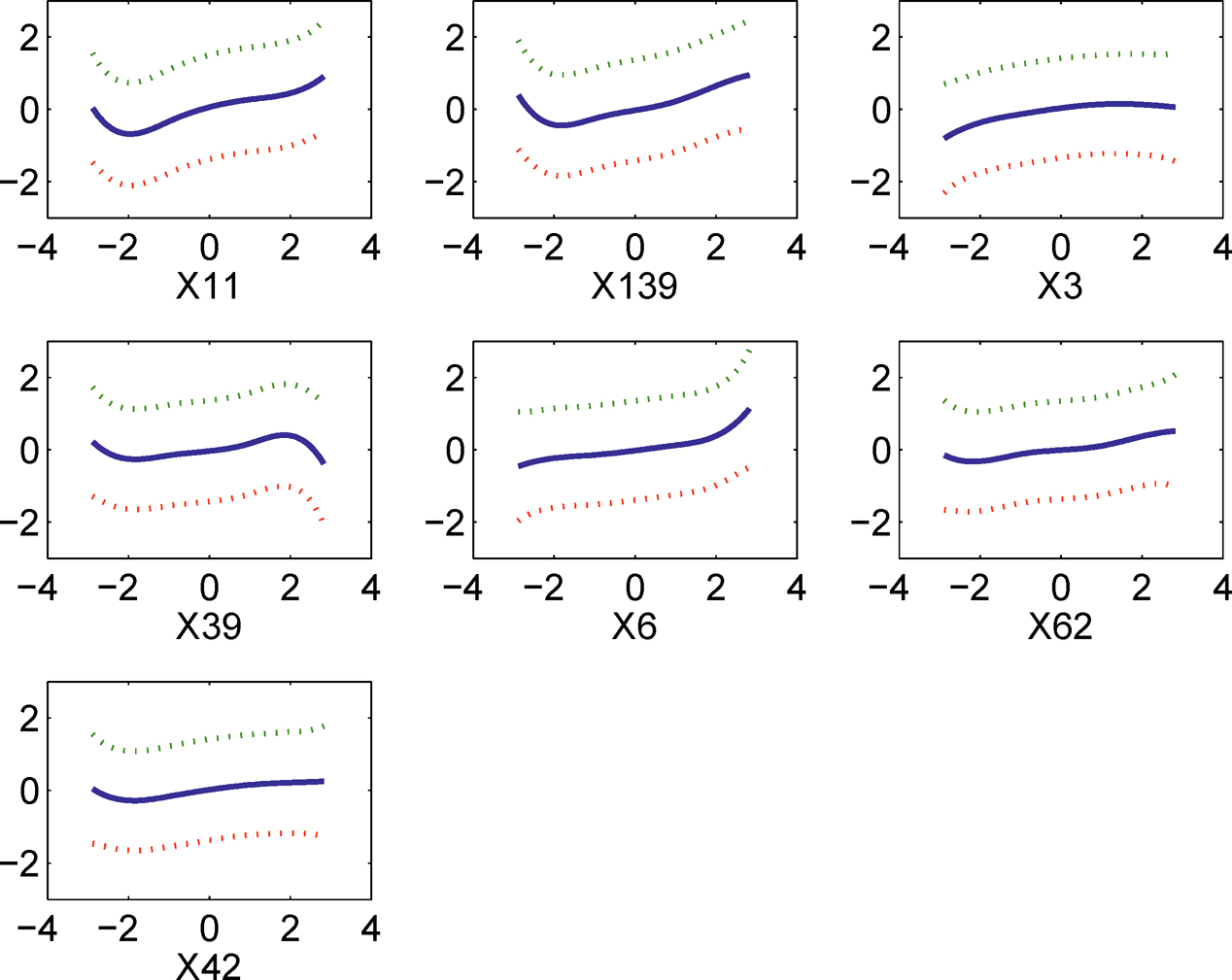
Figure 8.6: Estimated functions based on 7 variables selected from 28 variables that survive DC-SIS screening by the x2-test with the RCV error variance estimator. Taken from Chen, Fan and Li (2018).
For a linear regression model Y = XTβ +ε, let β be the least squares estimate of β. The linear predictor Ŷ = xTβ̂ has prediction error at a new observation {x, Y*}: E{ (Y, - xTβ̂)2 |X, x*} = σ2(1 + xT* (xTX)-1x*), where σ2 is the error variance. This explains why the MSPE is slightly greater than σ̂2RCV. To further gauge the accuracy of the RCV estimate of σ2, define the weighted prediction error |y* - xT* β̂ |/ √1+xT* (XTX)-1X*. Then the leave-one-out method leads to the mean squared weighted predictor error (MSWPE) 0.1289 and the average of the five-fold CV based on 400 randomly splitting data yields MSWPE 0.1305 with the 2.5th percentile and 97.5th percentile being 0.1254 and 0.1366, respectively. These results imply (a) the seven selected variables achieves the benchmark prediction; (b) the modeling biases using the additive models of these seven variables are negligible; (c) acv provides a very good estimate for σ2.
Their estimated functions m̂j/ (xj) are depicted in Figure 8.6, from whichit seems that all predictors shown in Figure 8.6 are not significant since zero crosses the entire confidence interval. This can be due to the fact that we have used too many variables which increases the variance of the estimate.

Figure 8.7: Estimated functions based on 2 variables selected from 28 variables that survive DC-SIS screening by the χ2-test with the RCV error variance estimator and the Bonferroni adjustment. Taken from Chen, Fan and Li (2018).
We further employ the Wald’s test with Bonferroni correction for 28 null hypotheses. This leads to only two significant predictors, X11 and X6, at level 0.05. We refit the data with the two selected predictors. Figure 8.7 depicts the plot of m̂11(x11) and m̂6(x6).
8.9 Bibliographical Notes
Fan and Lv (2008) first proposed the concept of SIS for linear regression models. Hall and Miller (2009) proposed generalized correlation for feature screening and proposed using bootstrap to quantify the uncertainty of feature rankings. Li, Peng, Zhang and Zhu (2012) proposed a rank correlation based feature screening procedure to achieve the robustness. Fan and Fan (2008) apply the idea of SIS for binary classification problems based on a two-sample t-statistic. Pan, Wang and Li (2016) proposed a feature screening procedure for multiclass linear discriminant analysis based on partial residuals. Fan, Samworth and Wu (2009) developed a feature screening procedure under a general parametric framework. Fan and Song (2010) proposed using the marginal likelihood estimate for feature screening in generalized linear models. Fan, Feng and Wu (2012) extended the idea of Fan and Song (2010) to the partial likelihood setting for survival data. Zhao and Li (2012) proposed using the marginal t-statistic derived from marginal partial likelihood estimate for feature screening in high dimensional survival data. Xu, Zhu and Li (2014) developed a feature screening procedure for longitudinal data based on the generalized estimating equation method.
There are many publications on feature screening for nonparametric and semiparametric models. Fan, Feng and Song (2011) extended the SIS for high dimensional additive models by using spline regression techniques. Liu, Li and Wu (2014) developed a SIS procedure for varying coefficient models based on conditional Pearson correlation. Fan, Ma and Dai (2014) further used spline regression techniques for high dimensional varying coefficient models. Song, Yi and Zou (2014) and Chu, Li and Reimherr (2016) developed two feature screening procedures for varying coefficient models with longitudinal data. Cheng, Honda, Li and Peng (2014) developed an automatic procedure for finding a sparse semi-varying coefficient models in the longitudinal data analysis. Extending the forward regression for ultrahigh dimensional linear model in Wang (2009), Cheng, Honda and Zhang (2016) proposed using forward regression for feature screening in ultrahigh dimensional varying coefficient models and studied its theoretical property. Li, Ke and Zhang (2015) proposed using penalized likelihood methods for structure specification in high-dimensional generalized semi-varying coefficient models. Chu, Li, Liu and Reimherr (2020) developed a feature screening procedure for generalized varying coefficient mixed effect models.
Model-free feature screening was first proposed in Zhu, Li, Li and Zhu (2011) for multi-index regression models. Based on Zhu et al, (2011), Lin, Sun and Zhu (2013) proposed a nonparametric feature screening for multi-index models. He, Wang and Hong (2013) proposed a model-free feature screening procedure using quantile regression techniques. Ma, Li and Tsai (2017) further developed partial quantile correlation for feature screening. Li, Zhong and Zhu (2012) introduced ideas of a test of independence for feature screening and proposed a feature screening procedure based on distance correlation. Mai and Zou (2013) proposed using the Kolmogorov statistic for a test of independence in the literature of goodness of fit as a marginal utility for feature screening in high dimensional binary classification. Mai and Zou (2015) further developed the fused Kolmogorov filter for model-free feature screening with multicategory, counts and continuous response variables. Cui, Li and Zhong (2014) developed a statistic to measure the independence between a continuous random variable and a categorical random variable and further using this statistic as a marginal utility for feature screening in discriminant analysis. Huang, Li and Wang (2014) employed the Pearson χ2-test statistic for independence as a marginal utility for feature screening when the response and covariates are categorical. Wang, Liu, Li and Li (2017) developed a model-free conditional independence feature screening procedure and established the sure screening property and consistency in ranking property under a set of regularity conditions. Zhou, Zhu, Xu and Li (2019) developed a new metric named cumulative divergence (CD), and further proposed a CD-based forward screening procedure, which is also a model-free forward screening procedure.
The idea of using data splitting for improving statistical inference may go back to Cox (1975). Wasserman and Roeder (2009) suggested using data splitting in high dimensional variable selection to achieve valid statistical inference after model selection. Fan, Guo and Hao (2012) proposed refitted cross-validation for error variance estimation. Unlike the procedure in Wasserman and Roeder (2009), which uses only parts of data for statistical inference, the refitted cross-validation method uses all data for estimation of error variance. Chen, Fan and Li (2018) developed the refitted cross-validation method for high dimensional additive models.
8.10 Exercises
8.1 Construct an example of a linear regression model, in which for some j, X3 is jointly dependent but marginally independent with the response Y.
8.2 Based on the relation between the Pearson correlation and the Kendall τ correlation under normality assumption, show that the screening procedures based on the Pearson correlation and the rank correlation are equivalent for ultrahigh dimensional normal linear models.
8.3 For ultrahigh dimensional linear regression models, show that under some conditions, the screening procedure in (8.12) is equivalent to the SIS based on the Pearson correlation proposed in Section 8.1. Further show the marginal utility Lj defined in Section 8.3.2 is also equivalent to the SIS based on the Pearson correlation for ultrahigh dimensional linear models.
8.4 Let Y be the response along with a continuous covariate U and covariate vector X = (X1, ,Xp)T. Partial linear model is defined by

where β0(·) is the unknown baseline function. Construct a sure independent screening procedure by applying related techniques to screening procedures for varying coefficient models studied in Section 8.4.2.
8.5 Construct sure screening procedures in Section 8.5.3 for the settings in which the response Y is continuous, while X consists of categorical covariates such as SNPs in a genome wise association study.
8.6 Refer to Section 8.6.2. Show that h(β; β(t)) =ln(β) and h(β; β(t)) ≥ ln(β) for any β with a proper chosen u. Further establish the ascent property of the IHT algorithm.
8.7 Prove Theorem 8.5.
8.8 A cardiomyopathy microarray data set can be downloaded from this book website. This data set was once analyzed by Segal, Dahlquist and Conklin (2003), Hall and Miller (2009) and Li, Zhong and Zhu (2012). The data set consists of n = 30 samples, each of which has p = 6319 gene expressions. The goal is to identify the most influential genes for overexpression of a G protein-coupled receptor (Ro1) in mice. The response Y is the Rol expression level, and the predictors Xks are other gene expression levels.
(a) Apply the Pearson correlation marginal screening procedure introduced in Section 8.1 to this data set.
(b) Apply the generalized correlation marginal screening procedure introduced in Section 8.2 to this data set.
(c) Apply the DC-SIS procedure introduced in Section 8.5.2 to this data.
(d) Comment upon your findings in (a), (b) and (c).
8.9 The data set ‘Rat Eye Expression.txt’ consists of microarray data of tissue harvesting from the eyes of a 120 twelve-week-old male rat. The microarrays are used to analyze the RNA from the eyes of these rats. There are 18,976 probes for each rat in this data set, which was used by Scheetz, et al. (2006) and Huang, Ma and Zhang (2008), and re-analyzed by Li, Zhong and Zhu (2012) for illustrating their iterative DC-SIS. The data can be downloaded from this book’s website. Following Huang, Ma and Zhang (2008), take the response variable to be TRIM32, which is one of the selected 18,976 probes and corresponds to the row with probe.name “1389163_at”.
(a) Select 3,000 probes with the largest variances from the 18,975 probes.
(b) Apply the DC-SIS in Section 8.5.2 to the regression model with the response TRIM32 and the selected 3,000 covariates.
(c) Apply the iterative DC-SIS in Section 8.5.2 to the regression model with the response TRIM32 and the selected 3,000 covariates
(d) Compare your findings in (b) and (c).