As mentioned in the introduction of Chapter 10, the dependence of high-dimensional measurements is often driven by several common factors: different variables have different dependence on these common factors. This leads to the factor model (10.4):
 (11.1)
for each component j =1, … ,p. These factors f can be consistently estimated by using the principal component analysis as shown in the previous chapter.
This chapter applies the principal component analysis and factor models to solve several statistics and machine learning problems. These include factor adjustments in high-dimensional model selection and multiple testing and high-dimensional regression using augmented factor models. Principal component analysis is a form of spectral learning. We also discuss other applications of spectral learning in problems such as matrix completion, community detection, and item ranking, and applications that serve as initial values for non-convex optimization problems such as mixture models. Detailed treatments of these require a whole book. Rather, we focus only on some methodological powers of spectral learning to give the reader some idea of its importance to statistical machine learning. Indeed, the role of PCA in statistical machine learning is very similar to regression analysis in statistics.
11.1 Factor-adjusted Regularized Model Selection
Model selection is critical in high dimensional regression analysis. Numerous methods for model selection have been proposed in the past two decades, including Lasso, SCAD, the elastic net, the Dantzig selector, among others. However, these regularization methods work only when the covariates satisfy certain regularity conditions such as the irrepresentable condition (3.38). When covariates admit a factor structure (11.1), such a condition breaks down and the model selection consistency can not be granted.
11.1.1 Importance of factor adjustments
As a simple illustrative example, we simulate 100 random samples of size n = 100 from the p= 250 dimensional sparse regression model
 (11.2)
where X ~ N(0, Σ) and Σ is a compound symmetry correlation matrix with equal correlation ρ. We apply Lasso to each sample and record the average model size and the model selection consistency rate. The results are depicted in Figure 11.1. The model selection consistency rate is low for Lasso when ρ≥ 0.2, due to over estimation of model size.
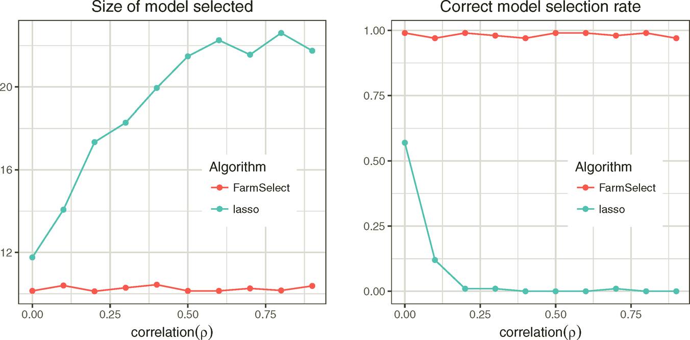
Figure 11.1: Comparison of model selection consistency rates by Lasso with (FarmSelect) and without (Lasso) factor adjustments.
The failure of model selection consistency is due to high correlation among the original variables X in p dimensions. If we use the factor model (11.1), the regression model (11.2) can now be written as
 (11.3)
where α = aTβ and γ= BTβ. If u and f were observable, we obtain a (p + 1 + K)-dimensional regression problem if γ and α are regarded as free parameters. In this lifted space, the covariates f and u are now weakly correlated (indeed, they are independent under specific model (11.2)) and we can now apply a regularized method to fit model (11.3). Note that the high-dimensional coefficient vector β in (11.3) is the same as that in (11.2) and is hence sparse.
In practice, u and f are not observable. However, they can be consistently estimated by PCA as shown in Section 10.5.4. Regarding the estimated latent factors {fi}i=1n and the idiosyncratic components {ui} as the covariates, we can now apply a regularized model selection method to the regression problem (11.3). The resulting method is called a Factor-Adjusted Regularized Model selector or FarmSelect for short. It was introduced by Kneip and Sarda (2011) and expanded and developed by Fan, Ke and Wang (2020). Figure 11.1 shows the effectiveness of FarmSelect: The model selection consistency rate is nearly 100%, regardless of ρ.
Finally, we would like to remark in representation (11.3), the parameter γ = BTβ is not free (B is given by the factor model). How can we assure that the least-squares problem (11.3) with free γ would yield a solution γ = BTβ? This requires the condition
 (11.4)
See Exercise 11.1. This is somewhat stronger than the original condition that EXε = 0 and holds easily as X is exogenous to ε.
11.1.2 FarmSelect
The lifting via factor adjustments is used to weaken the dependence of covariates. It is insensitive to the over-estimate on the number of factors, as the expended factor models include the original factor models as a specific case and hence the dependence of new covariates has also been weakened. The idea of factor adjustments is more generally applicable to a family of sparse linear model
 (11.5)
following a factor model, where g(.,.) is a known function. This model encompasses the generalized linear models in Chapter 5 and proportional hazards model in Chapter 6.
Suppose that we fit model (11.5) by using the loss function L(Yi, XiT β), which can be a negative log-likelihood. This can be the log-likelihood function or M-estimation. Instead of regularizing directly via
 (11.6)
where pλ(·) is a folded concave penalty such as Lasso, SCAD and MCP with a regularization parameter λ, the Factor-Adjusted Regularized (or Robust when so implemented) Model selection (FarmSelect) consists of two steps:
• Factor analysis. Obtain the estimates of fi and ûi in model (11.5) via PCA.
• Augmented regularization. Find α, β and γ to minimize
 (11.7)
The resulting estimator is denoted as β. The procedure is implemented in R package FarmSelect. Note that the β in augmented model (11.7) is the same as that in model (11.5).
As an illustration, we consider the sparse linear model (11.2) again with p = 500 and β = (β1,, β10, 0p−10)T, where {β}j=1 are drawn uniformly at random from [2, 5]. Instead of taking the equi-correlation covariance matrix, the correlation structure is now calibrated to that for the excess monthly returns of the constituents of the S&P 500 Index between 1980 and 2012. Figure 11.2 reports the model selection consistency rates for n ranges 50 to 150. The effectiveness of factor adjustments is evidenced.

Figure 11.2: FarmSelect is compared with Lasso, SCAD, Elastic Net in terms of selection consistency rates. Taken from Fan, Ke and Wang (2020).
As pointed out in Fan, Ke and Wang (2020), factor adjustments can also be applied to variable screening. This can be done via an application of an independent screening rule to variables u or by the conditional sure independent screening rule, conditioned on the variables f. See Chapter 8 for details.
11.1.3 Application to forecasting bond risk premia
As an empirical application, we take the example in Fan, Ke, Wang (2019+) that predicts the U.S. government bond risk premia by a large panel of macroeconomic variables mentioned in Section 1.1.4. The response variable is the monthly data of U.S. bond risk premia with maturity of 2 to 5 years between January 1980 and December 2015, consisting of 432 data points. The bond risk premia is calculated as the one year return of an n years maturity bond excessing the one year maturity bond yield as the risk-free rate. The co-variates are 131 monthly U.S. disaggregated macroeconomic variables in the FRED-MD database1. These macroeconomic variables are driven by economic fundamentals and are highly correlated. To wit, we apply principal component analysis to these macroeconomic variables and obtain the scree plot of the top 20 principal components in Figure 11.3. It shows the first principal component alone explains more than 60% of the total variance. In addition, the first 5 principal components together explain more than 90% of the total variance.
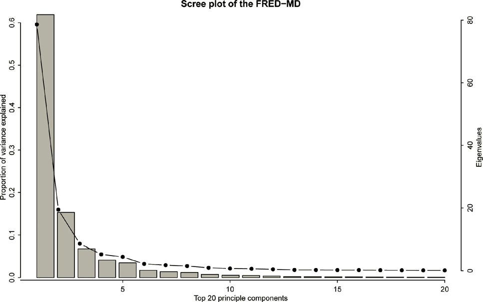
Figure 11.3: Eigenvalues (dotted line) and proportions of variance (bar) explained by the top 20 principal components for the macroeconomic data. Taken from Fan, Ke and Wang (2020).
We forecast one month bond risk premia using a rolling window of size 120 months. Within each window, the risk premia is predicted by a sparse linear regression of dimensionality 131. The performance is evaluated by the out-of-sample R, defined as
where yt is the response variable at time t, Ŷt is the predicted Yt using the previous 120 months data, and Yt is the sample mean of the previous 120 months responses (Yt−120, …,Yt−1), representing a naive baseline predictor.
We compare FarmSelect with Lasso in terms of prediction and model size. We include also the principal component regression (PCR), which uses f as predictors, in the prediction competition. The FarmSelect is implemented by the R package FarmSelect with default settings. To be specific, the loss function is L1, the number of factors is estimated by the eigen-ratio method and the regularized parameter is selected by multi-fold cross validation. The Lasso method is implemented by the glmnet R package. The PCR method is implemented by the pls package in R. The number of principal components is chosen as 8 as suggested in Ludvigson and Ng (2009).
_______________
1 The FRED-MD is a monthly economic database updated by the Federal Reserve Bank of St. Louis which is publicly available at http://research.stlouisfed.org/econ/mccracken/sel/
Table 11.1: Out of sample R2 and average selected model size by FarmSelect, Lasso, and PCR.

Table 11.1, taken from Fan, Ke and Wang (2019+), reports the results. It is clear that FarmSelect outperforms Lasso and PCR, in terms of out-of-sample R, even though Lasso uses many more variables. Note that PCR always uses 8 variables, which are about the same as FarmSelect.
11.1.4 Application to a neuroblastoma data
Neuroblastoma is a malignant tumor of neural crest origin that is the most frequent solid extracranial neoplasia in children. It is responsible for about 15% of all pediatric cancer deaths. Oberthuer et al. (2006) analyzed the German Neuroblastoma Trials NB90-NB2004 (diagnosed between 1989 and 2004) and developed a classifier based on gene expressions. For 246 neuroblastoma patients, aged from 0 to 296 months (median 15 months), gene expressions over 10,707 probe sites were measured. We took 3-year event-free survival information of the patients (56 positive and 190 negative) as the binary response and modeled the response as a high dimensional sparse logistic regression model of gene expressions.
First of all, due to co-expressions of genes, the covariates are correlated. This is evidenced by the scree plot in Figure 11.4. The figure and the numerical results here are taken from an earlier version of Fan, Ke and Wang (2020). The scree plot shows the top ten principal components together can explain more than 50% of the total variance. The eigen ratio method suggests a K̂=4 factor model. Therefore, FarmSelect should be advantageous in selecting important genes.
FarmSelect selects a model with 17 genes. In contrast, Lasso, SCAD and Elastic Net (with λ1 = λ2 ≡ λ) select much larger models, including 40, 34 and 86 genes respectively. These methods over-fit the model as they ignore the dependence among covariates. The over fitted models make it harder to interpret the molecular mechanisms and biological processes.
To assess the performance of each model selection method, we apply a bootstrap based out-of-sample prediction as follows. For each replication, we randomly draw 200 observations as the training set and leave the remaining 46 data points as the testing set. We use the training set to select and fit a model. Then, for each observation in the testing set, we use the fitted model to calculate the conditional probabilities and to classify outcomes. We record the selected model size and the correct prediction rate (No. of correct predictions/46). By repeating this procedure over 2,000 replications, we report the average model sizes and average correct prediction rates in Table 11.2. It shows that FarmSelect has the smallest average model size and the highest correct prediction rate. Lasso, SCAD and Elastic Net tend to select much larger models and result in lower prediction rates. in Table 11.2 we also report the out-of-sample correct prediction rate using the first 17 variables that entered the solution path of each model selection method. As a result, the correct prediction rates of Lasso, SCAD and Elastic Net decrease further. This indicates that the Lasso, SCAD and Elastic Net are likely to select overfitted models.

Figure 11.4: : Eigenvalues (dotted line) and proportional of variance (bar) explained by the top 20 principal components for the neuroblastoma data.
Table 11.2: Bootstrapping model selection performance of neuroblastoma data
| Bootstrap sample average | Model selection methods | |||
| FarmSelect | Lasso | SCAD | Elastic Net | |
| Model size | 17.6 | 46.2 | 34.0 | 90.0 |
| Correct prediction rate | 0.813 | 0.807 | 0.809 | 0.790 |
| Prediction performance with first 17 variables entering the solution path | ||||
| FarmSelect | Lasso | SCAD | Elastic Net | |
| Correct prediction rate | 0.813 | 0.733 | 0.764 | 0.705 |
11.1.5 Asymptotic theory for FarmSelect
To derive the asymptotic theory for FarmSelect, we need to solve the following three problems:
1. Like problem (11.3), the unconstrained minimization of E L(Y, α + uTβ + fTγ) with respect to α, β and γ is obtained at
 (11.8)
under model (11.1).
2. Let θ = (α, βT, γT)T The error bounds ‖θ−θ*‖ℓ for ℓ= 1, 2, ∞ and sign consistency sgn(β̂) = sgn(β*) should be available for the M-estimator (11.7), when {(uiT, fi)T}i=1n were observable.
3. The estimation errors in {(ûiT, fi)T}i=1n are negligible for the penalized M-estimator (11.7).
Similar to condition (11.4), Problem 1 can be resolved by imposing a condition
 (11.9)
where ∇L(s, t) = ∂L(s,t)/∂t. See Exercise 11.2. Problem 2 is solved in Fan, Ke and Wang (2020) for strong convex loss function under the Li-penalty. Their derivations are related to the results on the error bounds and sign consistency for the Li-penalized M-estimator (Lee, Sun and Taylor, 2015). Problem 3 is handled by restricting the likelihood function to the generalized linear model, along with the consistency of estimated latent factors and idiosyncratic components in Sections 10.5.3 and 10.5.4. In particular, the representable conditions are now imposed based on u and f, which is much easier to satisfy. We refer to Fan, Ke and Wang (2019+) for more careful statements and technical proofs.
Finally, we would also to note that in the regression (11.7), only the linear space spanned by {fi}i=1n matters. Therefore, we only require the consistent estimation of the eigen-space spanned by {fi}i=1n, rather than consistency of each individual factors.
11.2 Factor-adjusted Robust Multiple Testing
Sparse linear regression attempts to find a set of variables that explain jointly the response variable. In many high-dimensional problems, we are also asking about individual effects of treatments such as which genes expressed differently within different cells (e.g. tumor vs. normal control), which mutual fund managers have positive α-skills, namely, risk-adjusted excess returns. These questions result in high-dimensional multiple testing problems that have been popularly studied in statistics. For an overview, see the monograph by Efron (2012) and reference therein.
Due to co-expression of genes or herding effect in fund management as well as other latent factors, the test statistics are often dependent. This results in a correlated test whose false discovery rate is hard to control (Efron, 2007, 2010; Fan, Han, Gu, 2012). Factor adjustments are a powerful tool for this purpose.
11.2.1 False discovery rate control
Suppose that we have n measurements from the model
 (11.10)
Here Xi can be in one case the p-dimensional vector for the logarithms of gene expression ratios between the tumor and normal cells for individual i or in another case the risk adjusted returns. It can also be the risk-adjusted mutual fund returns over the ith period. Our interest is to test multiple times the hypotheses
 (11.11)
Let Tj be a generic test statistic for H0j with rejection region |Tj| ≥ z for a given critical value z > 0. Here, we implicitly assumed that the test statistic Tj has the same null distribution; otherwise the critical value z should be zj. The numbers of total discoveries R(z) and false discoveries V(z) are the number of rejections and the number of false rejections, defined as
 (11.12)
Note that R(z) is observable, which is really the total number of rejected hypotheses, while V(z) needs to be estimated, depending on the unknown set

which is also called true null. The false discovery proportion and false discovery rate are defined respectively as
 (11.13)
with convention 0/0=0. Our goal is to control the false discovery proportion or false discovery rate. The FDP is more relevant for the current data. But the diference is small when the test statistics are independent and p is large. Indeed, by the law of large numbers, under mild conditions,

However, the difference can be substantial when the observed data are dependent, as can be seen in Example 11.1.
Let Pj be the P-value for the jth hypothesis and P(1) ≤ … P(p) be the ordered p-values. The significance of the jth hypothesis (or the importance of the jth variable) is sorted by their p-values: the smaller the more importance. To control the false discovery rate at a prescribed level α, Benjamini and Hochberg (1995) propose to choose
 (11.14)
and reject all null hypotheses H0;(j) for j = 1; …, k̂. They prove such a procedure controls FDR at level α, under the independence assumption of P-values. The procedure can also be implemented by defining the Benjamini-Hochberg adjusted p-value:
 (11.15)
where the minimum is taken to maintain the monotonic property, and rejects the null hypotheses with adjusted P-value less than α. The function p. adjust in R implements the procedure.
To better understand the above procedure, let us express the testing procedure in terms of P-values: reject H0j when Pj ≤ t for a given significant level t. Then, the total number of rejections and total number of false discoveries are respectively
 (11.16)
and the false rejection proportion of the test is FDP(t)=v(t)/r(t) Note that under the null hypothesis, Pj is uniformly distributed. If the test statistics {Tj} are independent, then the sequence {I(Pj < t)} are the i.i.d. Bernoulli random variable with the probability of success t. Thus, v(t) ≈ pot, where p0=|S0| is the number of true nulls. This is unknown, but can be upper bounded by p. Using this bound, we have an estimate
 (11.17)
The Benjamini-Hockberg method takes t = P(k̂) with k given by (11.14). Consequently,
by (11.14). This explains why the Benjamini-Hockberg approach controls the FDR at level α.
As mentioned above, estimating π0 =p0/p by its upper bound 1 will control the FDP correctly but it can be too crude. Let us now briefly describe the method for estimating π0 by Storey (2002). Now the histogram of P-values for the p hypotheses is available to us (e.g. Figure 11.5), which is a mixture of those from true nulls S0 and false nulls S0c. Assume P-values for false nulls (significant hypotheses) are all small so that P-values exceeding a given threshold η ∈ (0, 1) are all from the true nulls (e.g. η = 0.5). Under this assumption, π0 (1 −η) should be approximately the same as the percentage of P-values that exceed η. This leads to the estimator:
 (11.18)
for a given η= 0.5, say. Figure 11.7, taken from Fan, Wang, Zhong, Zhu, (2019+), illustrates the idea.
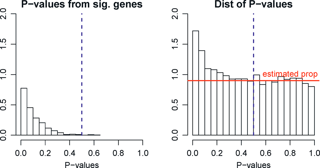
Figure 11.5: Estimation of proportion of true nulls. The observed P-values (right panel) consist of those from significant variables, which are usually small, and those from insignificant variables, which are uniformly distributed. Assuming the P-values for significant variables are mostly less than η (taken to be 0.5 in this illustration, left panel), the contributions of observed P-values > η are mostly from true nulls and this yields a natural estimator (11.20), which is the average height of the histogram with P-values > η (red line). Note that the histograms above the red line estimates the distributions of P-values from the significant variables in the left panel.
11.2.2 Multiple testing under dependence measurements
Due to co-expressions of genes and latent factors, the gene expressions in the vector Xi are dependent. Similarly, due to the “herding effect” and unadjusted latent factors, the fund returns within the ith period are correlated. This calls for further modeling the dependence in εi in (11.10).
A common technique for modeling dependence is the factor model. Modeling εi by a factor model, by (11.10), we have
 (11.19)
for all i= 1, …, n. In the presence of strong dependence, the FDR and FDP can now be very different, making the interpretation harder. The following example is adapted from Fan and Han (2017).
Example 11.1 To gain insight on how the dependence impacts on the number of false discoveries, consider model (11.19) with only one factor fi ~ N(0, 1) and B = ρ1 and ui~ N(0, (1 − ρ)Ip), namely,
Assume in addition that fi and ui are independent. The sample-average test statistics for problem (11.11) admit

where W =√nf̄ ~ N(0,1) is independent of U = √n/(1 − ρ)ū ~ N(0, Ip). Let p0 = |S0| be the size of true nulls. Then, the number of false discoveries

where a = (1 −ρ)−1/2 By using the law of large numbers, conditioning on W, we have as p0 → ∞ that

Therefore, the number of false discoveries depends on the realization of W. When ρ=0, p0−1 V(z) ≈2 Φ(−z). In this case, the FDP and FDR are approximately the same. To quantify the dependence on the realization of W, let p0=1000 and z=2.236 (the 99th percentile of the normal distribution) and ρ=0.8 so that

When W = −3, −2, −1,0, the values of p0−1 V(z) are approximately 0.608, 0.145, 0.008 and 0, respectively, which depend heavily on the realization of W. This is in contrast with the independence case in which p0−1 V(z) is always approximately 0.02.
11.2.3 Power of factor adjustments
Assume for a moment that B and fi are known in (11.19). It is then very natural to base the test on the adjusted data
 (11.20)
This has two advantages: the factor-adjusted data has weaker dependence since the idiosyncratic component ui is assumed to be so. This makes FDP and FDR approximately the same. In other words, it is easier to control type I errors. More importantly, Yi has less variance than Xi. In other words, the factor adjustments reduce the noise without suppressing the signals. There-fore, the tests based on {Yi} also increase the power.
To see the above intuition, let us consider the following simulated example.

Figure 11.6: Histograms for the sample means from a synthetic three-factor models without (left panel) and with (right panel) factor adjustments. Factor adjustments clearly decrease the noise in the test statistics.
Example 11.2 We simulate a random sample of size n = 100 from a threefactor model (11.19), in which

with p = 100. We take μj=0.6 for j ≤ p/4 and 0, otherwise. Based on the data, we compute the sample average X. This results in a vector of p test statistics, whose histogram is presented in the left panel of Figure 11.6. The bimodality of the distribution is blurred by large stochastic errors in the estimates. On the other hand, the histogram (right panel of Figure 11.6) for the sample averages based on the factor-adjusted data {Xi− Bfi}i=1n reveals clearly the bimodality, thanks to the decreased noise in the data. Hence the power of the testing is enhanced. At the same time, the factor-adjusted data are now uncorrelated due to the removal of the common factors. If the errors u were generated from N(0, 3Ip), then the factor-adjusted data were independent and FDR and FDP are approximately the same.
We generated data from t3(0, Ip) to demonstrated further the power of robustification. The distribution has 3 — δ moment for any δ > 0, but is not sub- Gaussian. Therefore, we employ a robust estimation of means via the adaptive Huber estimator in Theorem 3.2. The resulting histograms of estimated means are depicted in Figure 11.7. It demonstrates that the robust procedure helps further reduce the noise in the estimation: the bimodality is more clearly re- vealed.
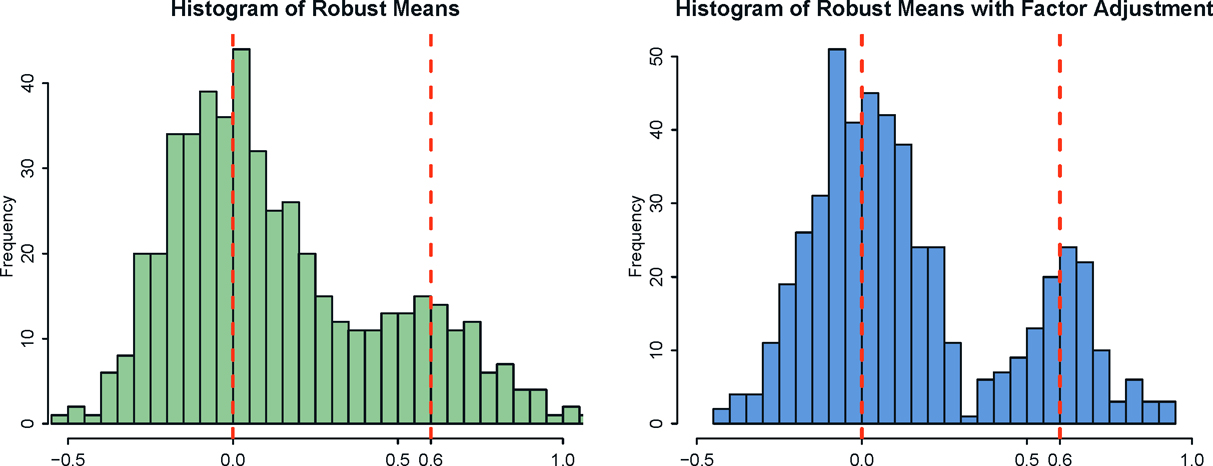
Figure 11.7: Histograms for the robust estimates of means from a synthetic three-factor models without (left panel) and with (right panel) factor adjustments. Factor adjustments clearly decreases the noise and robustness enhances the bimodality further.
11.2.4 FarmTest
The factor-adjusted test essentially applies a multiple testing procedure to the factor-adjusted data Yi in (11.20). This requires first to learn Bfi via PCA, apply the t-test to Yi, and then control FDR by the Benjamini-Hochberg procedure. In other words, the existing software is fed by using the factor-adjusted data {Yi}i=1n rather than the original data {Xi}i=1n.
The Factor Adjusted Robust Multiple test (Farm Test), introduced by Fan, Ke, Sun and Zhou (2019+), is a robust implementation of the above basic idea. Instead of using the sample mean, we use the adaptive Huber estimator to estimate μj for j= 1, … ,p. With a robustification parameter τj > 0, we consider the following M-estimator of μj:

where ρτ(u) is the Huber loss given in Theorem 3.2. It was then shown in Fan, Ke, Sun, Zhou (2018) that

where bjT is the jth row of B and f̄ =n−1 Σi=1n fi, and
 (11.21)
By (11.19), unknown f can be estimated robustly from the regression problem
 (11.22)
if {bj} are given, by regarding sparse {μj}pj=1 as outliers. Thus, given a robust estimate B̂, we obtain the robust estimate of f̂ for f by using (11.22) and use the factor adjusted statistic
where σ̂u,j is a robust estimator of σu,j. This test statistic is simply a robust version of the z-test based on the factor-adjusted data {Yi}.
We expect that the factor-adjusted test statistic Tj is approximately normally distributed. Hence, by the law of large numbers, the number of false discoveries
This is due to the fact that we assume that the correlation matrix of the idiosyncratic component vector ui is sparse so that {Ti}are nearly independent. Therefore, by definition (11.13), we have FDP(z) ≈ FDPA(z), where
 (11.23)
where π0 = p0/p. Note that FDPA(z) is nearly known, since only π0 is unknown. In many applications, true discoveries are sparse so that π0≈1. It can also be consistently estimated by (11.18).
We now summarize the FarmTest of Fan, Ke, Sun, Zhou (2019+). The inputs include {Xi}i=1n, a generic robust covariance matrix estimator Σ ∈ IRp×p from the data, a pre-specified level α ∈ (0, 1) for FDP control, the number of factors K, and the robustification parameters γ and {τj}i=1p. Many of those parameters can be simplified in the implementation. For example, K can be estimated by the methods in Section 10.2.3, and overestimating K has little impact on final outputs. Similarly, the robustification parameters {τj} can be selected via a five-fold cross-validation with their theoretically optimal orders taken into account.
FarmTest consists of the following three steps.
a) Compute the eigen-decomposition of Σ, set {λj}j=1K to be its top K eigen-values in descending order, and {v̂j}j=1K to be their corresponding eigen-vectors. Let B̂ (λ̃11/2v̂1,…,λ̃K1/2v̂K)∈IRp×K where λ̃j=max{λ̃j,0}, and denote its rows by {bj}j=1p.
b) Let x̄j = 1/n Σi=1n xij for j =1, … , p and f =argmaxf∈IRK Σj=1p ℓγ(x̄j− bjTf), which is an implementation of (11.22) by regarding sparse {μj} as “outliers”. Construct factor-adjusted test statistics
 (11.24)
where σ̂u,jj = θj−μ̂j ‖bj‖2, θj =arg minθj−μ̂j2 ‖bj‖2 ℓτj (xij-θ). This estimate of variance is based on (11.21).
c) Calculate the critical value zα= inf{z ≥ 0 : FDPA(z) ≤ α}, where FDPA(z) =2π̂0pΦ(−z)/R(z) (see (11.23)), and reject H0j whenever |Tj | > zα.
Step c) of FarmTest is similar to controlling the FDR by the Benjamini-Hockberg procedure, as noted in Section 11.2.1. Even though many heuristics are used in the introduction of the FarmTest procedure, the validity of the procedure has been rigorously proved by Fan, Ke, Sun, and Zhou (2019+). The proofs are sophisticated and we refer readers to the paper for details. The R software package FarmTest implements the above procedure.
In the implementation, Fan, Ke, Sun and Zhou (2019+) propose to use the robust U-covariance (9.28) or elementwise robust covariance (9.25) as their robust covariance matrix estimator Σ. They provide extensive simulations to demonstrate the advantages of the FarmTest. They showed that FarmTest controls accurately the false discovery rate and has higher power in improving missed discovery rates, in comparison to the methods without factor adjustments. They also show convincingly that when the error distribution ui has light tails, FarmTest performs about the same as its non-robust implementation; whereas when ui has heavy tails, FarmTest outperforms.
11.2.5 Application to neuroblastoma data
We now revisit the neuroblastoma data used in Section 11.1.4. The figures and the results are taken from Fan, Ke, Sun and Zhou (2019+). Instead of examining the joint effect via the sparse logistic regression, we now investigate the marginal effect: which genes expressed statistically differently in the neuroblastoma from the normal controls. The dependence of gene expression has been demonstrated in Figure 11.4. Indeed, the top 4 principal components (PCs) explain 42.6% and 33.3% of the total variance for the positive and negative groups, respectively.
Another stylized feature of high-dimensional data is that many variables have heavy tails. To wit, Figure 11.8 depicts the histograms of the excess kurtosis of the gene expressions for both positive (event-free survivals) and negative groups. For the positive group, the left panel of Figure 11.8 shows that 6518 gene expressions have positive excess kurtosis and 420 of them have kurtosis greater than 6. In other words, about 4% of gene expressions are severely heavy tailed as their tails are fatter than the t-distribution with 5 degrees of freedom. Similarly, in the negative group, 9341 gene expressions exhibit positive excess kurtosis with 671 of them have kurtosis greater than 6. Such a heavy-tailed feature indicates the necessity of using robust methods to estimate the mean and covariance of the data.
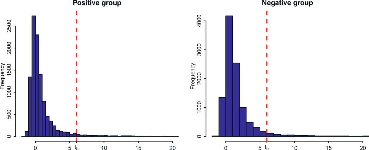
Figure 11.8: : Histograms of excess kurtosises for the gene expressions in positive and negative groups of the neuroblastoma data. The vertical dashed line shows the excess kurtosis (equals 6) of t5-distribution.
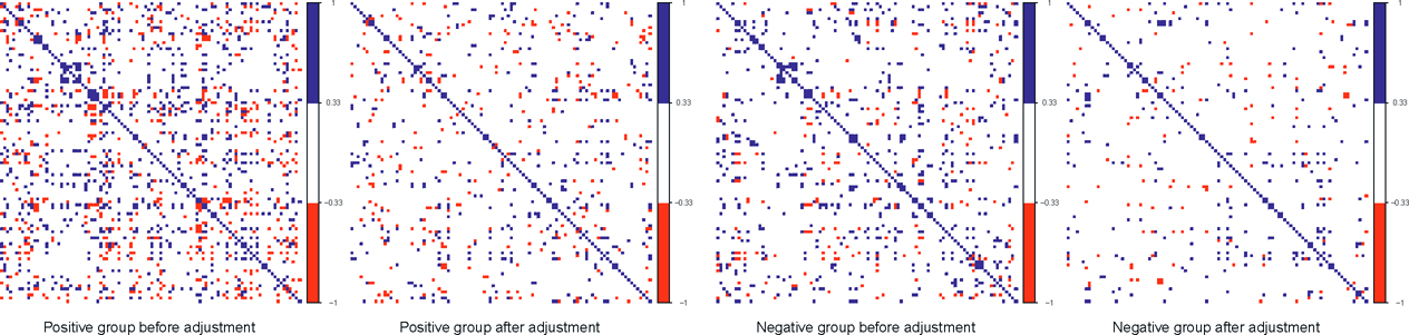
Figure 11.9: Correlations among the first 100 genes before and after factor adjustments. The blue and red pixels represent the pairs of gene expressions whose correlations are greater than 1/3 or less than —1/3, respectively.
The effectiveness of the factor adjustments is evidenced in Figure 11.9. Therefore, for each group, we plot the correlation matrices of the first 100 gene expressions before and after adjusting the top 4 PCs. It shows convincingly that the correlations are significantly weakened after the factor adjustments. More specifically, the number of pairs of genes with absolute correlation bigger than 1/3 drops from 1452 to 666 for the positive group and from 848 to 414 for the negative group.
The two-sample version of FarmTest uses the following two-sample t-type statistics:
 (11.25)
where the subscripts 1 and 2 correspond to the positive and negative groups, respectively. Specifically, μ̂1j and μ̂2j are the robust mean estimators, and b̂1j b̂2j, f̂1 and f̂2 are robust estimators of the factors and loadings based on a robust covariance estimator. In addition, σ̂ 1u,jj and σ̂ 2u,jj are the robust variance estimators defined in (11.24).
We apply four tests to the neuroblastoma data set: FarmTest with covariance inputs (9.25) (denoted by FARM-H) and (9.28) (denoted FARM-U), the non-robust factor-adjusted version using sample mean and sample variance (denoted as FAM) and the naive method without factor adjustments and ro-bustification. At level α= 0.01, FARM-H and FARM-U methods identify, respectively, 3912 and 3855 probes with different gene expressions, among which 3762 probes are identical. This shows an approximately 97% similarity in the two methods. In contrast, FAM and the naive method discover 3509 and 3236 probes, respectively. Clearly, the more powerful method leads to more discoveries.
11.3 Factor Augmented Regression Methods
Principal component regression (PCR) is very useful for dimensionality reduction in high-dimensional regression problems. Factor models provide new prospects for understanding why such a method is useful for statistical modeling. Such factor models are usually augmented by other covariates, leading to augmented factor models. This section introduces Factor Augmented Regression Methods for Prediction (FarmPredict)
11.3.1 Principal component regression
Principal component analysis is very frequently used in compressing high-dimensional variables into a couple of principal components. These principal components can also be used for regression analysis, achieving the dimensionality reduction.
Why are the principal components, rather than other components, used as regressors? Factor models offer a new modeling prospective. The basic assumption is that there are latent factors that drive the independent variables and the response variables simultaneously, as is schematically demonstrated in Figure 11.10. Therefore, we extract the latent factors from the independent variables and use the estimated latent factors as the predictors for the response variables. The latent factors are frequently estimated by principal components. Since principal components are used as the predictors in the regression for y, it is called principal component regression (PCR).
To understand the last paragraph better, suppose that we have data {(Xi(Yi)}i=1n and Xi and Yi are both driven by the latent factors via
 (11.26)
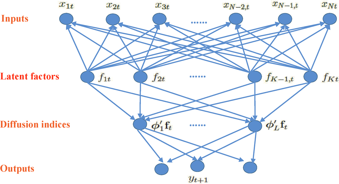
Figure 11.10: Illustration of principal components regression. Latent factors f1, …, fK drive both the input variables x1, …, xN and output variables y1, …, yq at time or subject t. The analysis is then to extract these latent factors via PCA and use these estimated factors f1, …, fK as predictors, leading to the principal component regression. An example of PCR is to construct multiple indices {øjT ft} of factors to predict Y; see (11.34).
where g(·) is a regression function. The model is also applicable in time series prediction, in which i indexes time t. Under model (11.26), we use data {Xi}i=1n to estimate {fi}i=1n via PCA, resulting in {f̂i}i=1n. We then fit the regression
 (11.27)
PCR corresponds to multiple regression in model (11.27):
 (11.28)
Due to the identifiability constraints of latent factors, we often normalize {fi}i=1n to have sample mean zero and sample variance identity. Under such a condition, the least-squares estimate admits the sample formula:
 (11.29)
where f̂ij is the jth component of fi, and K is the number of factors. Paul, Bair, Hastie and Tibshirani (2008) employed “preconditioning” (correlation screening) to reduce the dimensionality in learning latent factors.
PCR is traditionally motivated differently from ours. For simplicity, we assume that both the means of the covariates and the response are zero so that we do not need to deal with the mean. Write the linear model in the matrix form
Let X = UΔVT where Δ = diag(δ1, …, δp) is the diagonal matrix, consisting of its singular values, U = (u1, …, up) and V = (v1, …, vp) are the n × p and p × p orthogonal matrices, consisting of left- and right- singular vectors of matrix X. Then, the principal components based on the sample covariance matrix n−XTX are simply
where vj is the principal direction. Then, the PCR can be regarded as a constrained least-squares problem:
 (11.30)
The constraint can be regarded as regularization to reduce the complexity of β.
PCR also admits the optimality in the following sense. Let L be the p × (p − K) full rank matrix. Consider the generalization of the constrained least-squares problem (11.30)
 (11.31)
Let ß̂L be the solution and MSE(L) be the mean square error for estimating the true parameter vector β*. The optimal choice of L that minimizes the MSE is the one given by (11.30), or PCR (Park, 1981).
11.3.2 Augmented principal component regression
In many applications, we have more than one type of data. For example, in the macroeconomic data given in Section 11.1.3, in addition to 131 disaggregated macroeconomic data, we have 8 aggregated macroeconomics variables; see Section 11.3.3 for addition details. Similarly, in the neuroblastoma data in Section 11.1.4, in additional to the microarray gene expression data, we have demographical and clinical information such as age, weight, and social economic status, among others. Clearly these two types of variables can not be aggregated via PCA.
Assume that we have additional covariates Wi so that the observed data are now {(Wi, Xi,Yi)}ni=1. We assume that Wi is low-dimensional; otherwise, we will use the estimated common factors from Wi. The augmented factor model is to extract the latent factors {fi} from {Xi} and run the regression using both the estimated latent factors and the augmented variables:
 (11.32)
We will refer this class of prediction method to the Factor-Augmented Regression Model for Prediction or FarmPredict for short.
The regression problem in (11.32) can be a multiple regression model:
 (11.33)
This results in the augmented principal component regression. The regression function in (11.32) can also be estimated by using nonparametric function estimation such as the kernel and spline methods in Chapter 2 or deep neural network models in Chapter 14. It can also be estimated by using a multi-index model as is schematically shown in Figure 11.10. There, we attempt to extract several linear combinations of estimated factors, also called a diffusion index by Stock and Watson (2002b), to predict the response Y. See Fan, Xue and Yao (2017) for a study on this approach, which imposes the model:
 (11.34)
where X*i = (fTi, WTi)T is now the expanded predictors. In particular, when there is no Wi component, the model reduces to the case depicted in Figure 11.10.
Since the study of the multi-index model by Li (1991, 1992), there are a lot of developments in this area on the estimation of the diffusion indices. See Cook (2007, 2009) and the references therein.
11.3.3 Application to forecast bond risk premia
We now revisit the macroeconomic data presented in Section 11.1.3. In addition to the 131 disaggregated macroeconomic variables, we have 8 aggregated macroeconomic variables:
W1 = Linear combination of five forward rates;
W2 = GDP;
W3= Real category development index (CDI);
W4 = Non-agriculture employment;
W5 = Real industrial production;
W6 = Real manufacturing and trade sales;
W7= Real personal income less transfer;
W8 = Consumer price index (CPI)
These variables {Wt} can be combined with the 5 principal components {ft} extracted from the 131 macroeconomic variables to predict the bond risk premia. This yields the PCR based on covariates ft and the augmented PCR based on (WtT, ftT). The out-of-sample R2 for these two models is presented in the last block of Table 11.3 under the heading of PCA. The augmented PCR improves somewhat the out-of-sample R2, but not by a lot.
Another usage of the augmented variables Wt is to blend them in extracting the latent factors via projected PCA introduced in Section 10.4. It can be implemented robustly (labeled PPCA). After extracting the latent factors, we apply the multi-index model (11.34) to predict the bond risk premia. The diffusion indices coefficient {ϕj}Lj=1 is estimated via the slice inverse regression (Li, 1991) with the number of diffusion index L chosen by the eigen-ratio method. The choice is usually L = 2 or 3. The nonparametric function g in (11.34) is fitted by using the additive model g(x1, …, xL) = g1(x1) + … + gL(xL) via the local linear fit. The prediction results are shown in the first block of Table 11.3. It shows that extracting latent factors via projected PCA is far more effective than the augmented PCR. We also implemented a non-robust version of PPCA and obtained similar but somewhat weaker results than those by its robust implementation.
Table 11.3: Out-of-sample R2 (%) for linear prediction of bond risk premia. Adapted from Fan, Ke, and Liao (2018).
Table 11.4: Out-of-sample R2 (%) by the multi-index model for the bond risk premia. Adapted from Fan, Ke, and Liao (2018).
Fan, Ke, and Liao (2018) also applied the multi-index model to the PCA extracted factors along with the augmented variables. The out-of-sample R2 is presented in the second block of Table 11.4. It is substantially better than the linear predictor but is not as effective as the factors extracted by PPCA.
11.4 Applications to Statistical Machine Learning
Principal component analysis has been widely used in statistical machine learning and applied mathematics. The applications range from dimensionality reduction such as factor analysis, manifold learning, and multidimensional scaling to clustering analysis such as image segmentation and community detection. Other applications include item ranking, matrix completion, Z2-synchronization, and blind convolution and initialization for nonconvex optimization problems such as mixture models and phase retrieval. The role of PCA in statistical machine learning is very similar to that of regression analysis in statistics. It requires a whole book in order to give a comprehensive account on this subject. Rather, we only highlight some applications to give readers an idea of how PCA can be used to solve seemingly complicated statistical machine learning and applied mathematics problems.
In the applications so far, PCA is mainly applied to the sample covariance matrix or robust estimates of the covariance matrix to extract latent factors. In the applications below, the PCA is applied to a class of Wigner matrices, which are random symmetric (or Hermitian) matrices with independent elements in the upper diagonal matrix. It is often assumed that the random elements in the Wigner matrices have mean zero and finite second moment. In contrast, the elements in the sample covariance matrix are dependent. Factor modeling and principal components are closely related. We can view PCA as a form of spectral learning which is applied to the sample covariance matrix or robust estimates of the covariance matrix to extract latent factors.
11.4.1 Community detection
Community detection is basically a clustering problem based on network data. It has diverse applications in social networks, citation networks, genomic networks, economics and financial networks, among others. The observed network data are represented by a graph in which nodes represent members in the communities and edges indicate the links between two members. The data can be summarized as an adjacency matrix A (aij), where the element aij = 0 or 1 depends on whether or not there is a link between the ith and jth node.
The simplest probabilistic model is probably the stochastic block model, introduced in Holland and Leinhardt (1981), Holland, Laskey, and Leinhardt (1983) and Wang and Wong (1987). For an overview of recent developments, see Abbe (2018).
Definition 11.1 Suppose that we have n vertices, labeled {1, …, n}, that can be partitioned into K disjoint communities C1, …, CK. For two vertices k ∈ Ci and l ∈ Cj, a stochastic block model assumes that they are connected with probability pij, independent of other connections. In other words, the adjacency matrix A (Akl) is regarded as a realization of a sequence of independent Bernoulli random variables with
 (11.35)
The K × K symmetric matrix P = (pi,j) is referred to as the edge probability matrix.
In the above stochastic block model, the edge probability pij describes the connectivity between the two communities Ci and Cj. Within a community Ci, the connection probability is pii. The simplest model is the one in which pij = p for all i and j, and is referred to as the Erdös-Rényi graph or model (Erdös and Rényi, 1960). In other words, the partition is irrelevant, corresponding to a degenerate case, resulting in a random graph. Denote such a model as G(n, p).

Figure 11.11: Simulated network data from (a) Erdös-Rényi graph and (b) stochastic block model with n = 100, p = 5log(n)/n, and q = p/4. For SMB model, there were two communities, with the first n/2 members from group 1 and the second n/2 members from group 2; they are hard to differentiate because p and q are quite close.
A planted partition model corresponds to the case where pii = p for all i and pij = q for all i ≠ j and p ≠ q. In other words, the probability of within-community connections is p and the probability of between-community connections is q. When r = 2, this corresponds to the two community case. Figure 11.11 gives a realization from the Erdös-Rényi model and the stochastic block model. The simulations and plots are generated from the functions sample_gnp and sample_sbm in the R package igraph [install. package(“igraph”); library(igraph)].
Given an observed adjacency matrix A = (aij), statistical tasks include detecting whether the graph has a latent structure and recovering the latent partition of the communities. We naturally appeal to the maximum likelihood method. Let C(i) be the unknown community to which node i belongs. Then
the likelihood function of observing {aij}i>j is simply the multiplication of the Bernoulli likelihood:
where the unknown parameters are {C(i)}Ki=1 and P (pij) ∈ RK×K. This is an NP-hard computation problem. Therefore, various relaxed algorithms including semidefinite programs and spectral methods have been proposed; see Abbe (2018).
The spectral method is based on the method of moments. Let Γ be an n × K membership matrix, whose ith row indicates the membership of node i: It has an element 1 at the location C(i) and zero otherwise. The matrix Γ classifies each node into a community, with rows indicating the communities. Then, it is easy to see that E Aij = pC(i)C(j) for i ≠ j and
 (11.36)
except the diagonal elements, which are zero on the left (assuming no self-loop).2 It follows immediately that the membership matrix Γ falls in the eigen-space spanned by the first K eigenvectors of E A. Indeed, the column space of Γ is the same as the eigen-space spanned by the top K eigenvalues of E A, if P is not degenerate. See Exercise 11.9.
The above discussion reveals that the column space of Γ can be estimated via its empirical counterpart, namely the eigen-space spanned by the top K eigenvalues (in absolute value) of A. To find a consistent estimate of Γ, an unknown rotation is needed. This can be challenging to find. Instead of rotating, the second step is typically replaced by a clustering algorithm such as the K-means algorithm (see Section 13.1.1). This is due to the fact that if two members are in the same community, their corresponding rows of the eigen-vectors associated with the top K eigenvalues are the same, by using simple permutation arguments. See Example 11.3. Therefore, there are K distinct rows, which can be found by using the K-means algorithm. Spectral clustering is also discussed in Chapter 13. We summarize the algorithm for spectral clustering as in Algorithm 11.1.
Example 11.3 As a specific example, let us consider the planted partition model with two communities. For simplicity, we assume that we have two groups of equal size n/2. The first group is in the index set J and the second group is in the index set Jc. Then,
_______________
2 More rigorously, E A = ΓPΓT − diag(ΓPΓT). Since || diag(ΓPΓT) || ≤ maxk∈[K] pkk, this diagonal matrix is negligible in the analysis of the top K eigenvalues of E A under some mild conditions. Putting heuristically, EA ≈ ΓPΓT. We will ignore this issue throughout this section.
Algorithm 11.1 Spectral clustering for community detection
1. From the adjacency matrix A, get the n × K matrix Γ̂, consisting of the eigenvectors of the top K absolute eigenvalues;
2. Treat each of the n rows in Γ̂ as the input data, run a cluster algorithm such as k-means clustering to group the data points into K clusters. This puts n members into K communities. (Normalizing each rows to unit norm is recommended and is needed for more general situations)
has two non-vanishingeigenvalues. They are  and with corresponding eigenvectors
In this case, the sign of the second eigenvector identifies memberships. Our spectral method is particularly simple. Get the second eigenvector u2 from the observed adjacency matrix A and use sgn(u2) to classify each membership. Abbe, Fan, Wang and Zhong (2019+) show such a simple method is optimal in exact and nearly exact recovery cases.
We now apply the spectral method in Example 11.3 to the simulated data given in Figure 11.11. The results are depicted in Figure 11.12. From the screeplot in the left panel of Figure 11.12, we can see that the data from the Erdös-Rényi model has only one distinguished eigenvalue, whereas the data from the SBM model has two distinguished eigenvalues. This corresponds to the fact that E A is rank one for the Erdös-Rényi model and rank two for the SBM model. The right panel of Figure 11.12 demonstrates the effectiveness of the spectral method. Using the signs of the empirical second eigenvector as a classifier, we recover correctly the communities for almost all members based on the data generated from SBM. In contrast, as it should be, we only identify 50% correctly for the data generated from Erdös-Rényi model.
There are a number of variations on the applications of the spectral method. For each node, let be the degree of node i, which is the number of edges that node i has and D = diag(d1, …, dn) be the degree matrix. The Laplacian matrix, symmetric normalized Laplacian and random walk normalized Laplacian are defined as
 (11.37)
In step 1 of Algorithm 11.1, the adjacency matrix A can be replaced by one of the Laplacian matrices in (11.37). In step 2, the row of Γ̂ should be normalized to have the unit norm before running the K-mean algorithm. See Qin and Rohe (2013) and the arguments at the end of this subsection.
There are various extensions of the stochastic block models to make it more realistic. Mixed membership models have been introduced by Airoldi, Blei, Fienberg and Xing (2008) to accommodate members having multiple communities. Karrer and Newman (2011) introduced a degree corrected stochastic block model to account for varying degrees of connectivity among members in each community. We describe these models herewith to give readers some insights. We continue to use the notations introduced in Definition 11.1.
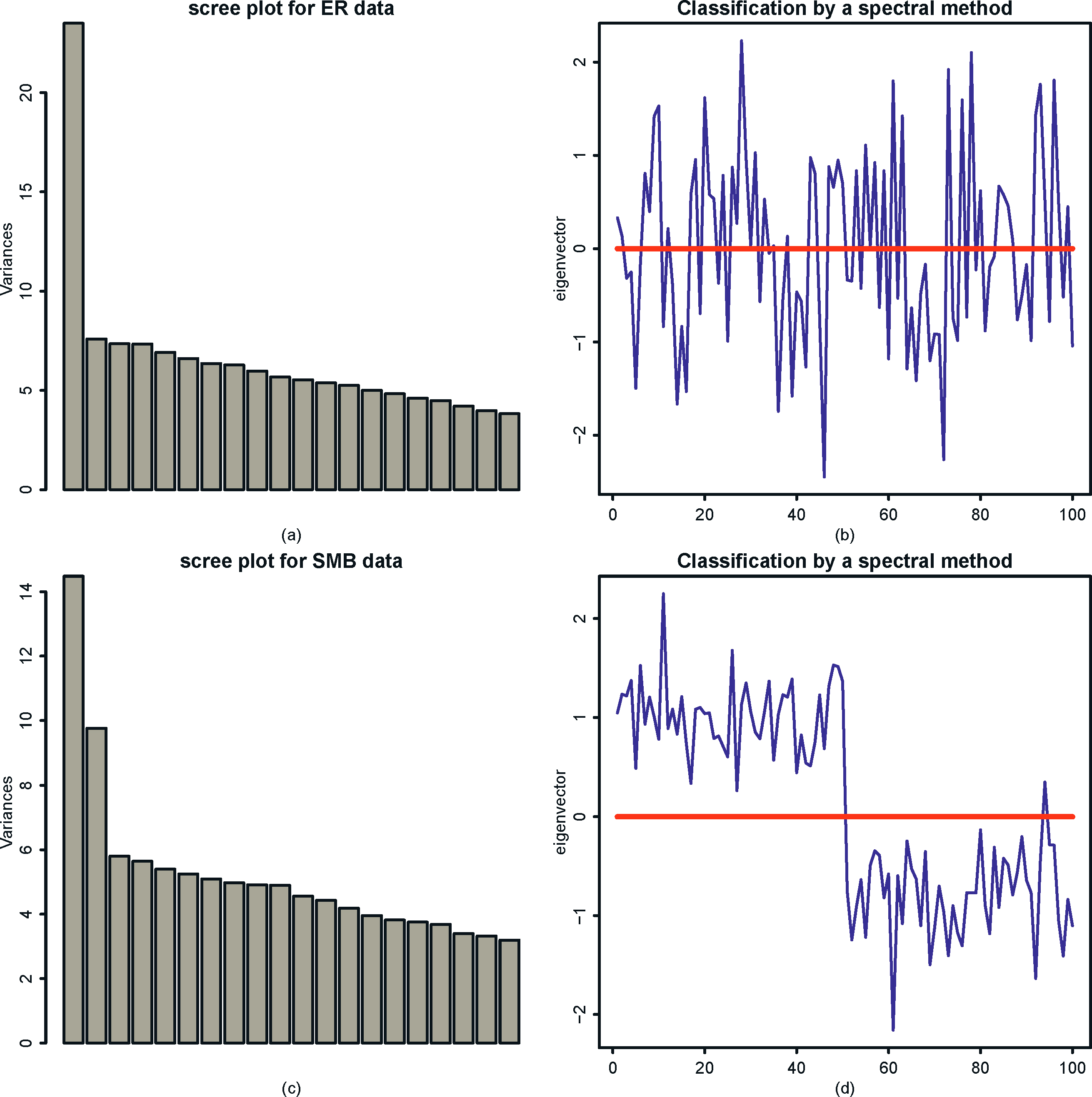
Figure 11.12: Spectral analysis for the simulated network data given in Figure 11.11. Top panel is for the data generated from the Erdös-Rényi model and the bottom is for the data generated from the stochastic block model. The left panel is the scree plot based on {|λi|}i=1 and the right panel is √nu2.
Definition 11.2 For each node i = 1, …, n, let πi be a K-dimensional probability vector that describes the mixed membership, with πi(k) = P(i ∈ Ck) for k ∈ [K] and θi > 0 representing the degree of heterogeneity in affinity of node i. Under the degree corrected mixed membership model, we assume that
 (11.38)
Here we implicitly assume that 0 ≤ θkθlpij ≤ 1 for all i, j, k and l. Consequently, the probability that there is an edge between nodes k and 1 is
 (11.39)
Note that when θi = 1 and πi is an indicator vector for all i = 1, …, n, model (11.39) reduces to the stochastic block model (11.35). If {θi} varies but πi is an indicator vector for all i = 1, …, n, we have the degree-corrected stochastic block model:
 (11.40)
Return to the general model (11.39). Let Θ = diag(θi, …, θn) then,
 (11.41)
where Π is an n × K matrix, with πiT as its ith row. Thus, ΘΠ falls in the space spanned by the eigenvectors of the top K eigenvalues of E A. They can be estimated by their empirical counterparts. A simple way to eliminate the degree heterogeneity Θ is the ratios of eigenvectors

where γ̂ik is the (i, k) element of Γ̂, the matrix of top K eigenvectors given in Algorithm 11.1. The community can now be detected by running the K-means algorithm on the rows {(Yi2, …,YiK)}ni=1. This is SCORE by Jin (2015). Another way to eliminate the degree heterogeneity is through normalization of rows of Γ̂ to the unit norm before running the K-mean algorithm.
To see why degree heterogeneity can be removed by the above two methods, let us consider the population version: E A or a symmetric normalized Laplacian version: (E D)−1/2 E A(E D)−1/2 (Note that L = D1/2LsymD1/2 falls also in this category). Whatever the version is used, the population matrix is of form Θ̇̃̃ΠPΠTΘ̇̃̃, where Θ̇̃ is a diagonal matrix. Let Γ be the matrix that comprises of the top K eigenvectors of Θ̇̃ΠPΠTΘ̇̃. Then, the column space spanned by Γ is the same as that spanned by Θ̇̃Π, assuming P is not degenerate. Therefore, there exists a nondegenerate K × K matrix V = (v1, …, vK) such that

where θ̃ = (θ̃1, …, θ̃n)T are the diagonal elements of Θ̃ and o is the Hadamard product (componentwise product). Let γj be the jth column of Γ. Then, the ratios of eigenvectors {γj/γ1}Kj=2 (componentwise division) will eliminate the parameter vector θ̃, resulting in {Πvj/Πv1}Kj=2. In addition, if Π has at most m distinct rows, so are the ratios of eigenvectors.
Similarly, letting {uiT}ni=1 be the rows of ΠV. Then, uiT = πTiV and the ith row of Γ is θ̃iuTi. If {πi}ni=1 have at most m distinct vectors, so do {ui}ni=1. Within a cluster, there might be different θ̃i but rows of Γ point the same direction ui = VTπi. Therefore, the normalization to the unit norm puts these rows at the same point so that the K-means algorithm can be applied.
Membership estimation by vertex hunting can be found in the paper by Jin, Ke and Luo (2017). Statistical inference on membership profiles πi is given in Fan, Fan, Han and Lv (2019).
11.4.2 Topic model
A topic model is used to classify a collection of documents into “topics” (see Figure 1.3). Suppose that we are given a collection of n documents and a bag of p words. Note that one of these words can be “none of the above words”. Then, we can count the frequencies of occurrence of p words in each document and obtain a p × n observation matrix D = (d1, …, dn), called the text corpus matrix, where dj is the observed frequencies of bag of words in document j. Suppose that there are K topics and the bag of words appears in topic k with a probability vector pk, k ∈ [K], with pik indicating the probability of word i in topic k. Like the mixed membership in the previous section, we assume that document j is a mixture of K topics with probability vector πj =(πj (1), …, πj(K))T, i.e. document j puts weight πj(k) on topic k. Therefore, the probability of observing the ith word in document j is

Let nj be the length of the jth document. We assume that

where d*j = (d*1j, …, d*pj)T. This is the probabilistic latent semantic indexing model introduced by Hofmann (1999).
Let Π be the n × K matrix with the jth row πTj,

Then, the observed data matrix D is related to unknown parameters through

which is of rank at most K. Let
be the singular value decomposition (SVD) of D*, where L* and R* are respectively the left and right singular vectors of D* and A* is the K × K diagonal matrix, consisting of K non-vanishing singular values. Then, the column space spanned by P is the same as that spanned by L*:
or P is identifiable by L* up to a right affine matrix U. Similarly,

The unknown matrix P and Π can be estimated by a spectral method. Let D = LAR be the SVD of the text corpus. Then L is an estimate of P up to a right K × K matrix U. This can be further identified by anchor words, a concept that is similar to the pure nodes in the mixed membership model. As explained at the end of Section 11.4.1, we can normalize the matrix D first, followed by post-SVD normalization. The K-means algorithm can be conducted by using different rows L for grouping words or R for clustering documents. We refer to Ke and Wang (2019) for details.
A popular Bayesian approach to topic modeling is the Latent Dirichlet Allocation, introduced by Blei, Ng and Jordan (2003), in which a Dirichlet prior on {πi} is imposed. The parameters are then estimated by a variational EM algorithm (Hoffman, Blei, Wang, and Paisley, 2013).
11.4.3 Matrix completion
A motivating example is the Netflix problem in movie-rating: Customer i rates movie j if she has watched the movie; otherwise the (i, j)-entry of the ratings matrix is missing. Since Netflix has millions of customers and tens of thousands of movies, most entries of the ratings matrix are missing. The task is to predict the remaining entries in order to make good recommendations to customers on what to watch next, namely to complete the matrix. Similar problems appear in ratings and recommendations for books, music and CDs, which are the basis for collaborative filtering in the recommender systems. Another example of matrix completion is the word-document matrix: The frequencies of words used in a collection of documents can be represented as a matrix and the task is to classify the documents.
Let Θ be the n1 × n2 true preference matrix that we would like to have: the preference score of the ith customer on the jth item. Instead, we observe only X on a small subset Ω of { 1, …, n1} × {1, …, n2}, which can possibly further be corrupted with noise (or uncertainties in ratings) so that the observed data are
 (11.42)
The problem as stated is under-determined even when there are no noises. What makes the solution feasible is the low-rank assumption of Θ. This assumption leads to the factor model interpretation. Take the movie rating as an example. Each movie has a number of features (factors) and different users have different loadings on these features plus some idiosyncratic components of personal tastes. This leads to the factor model (10.6) and low rank matrix Θ in (11.42). The main difference here is that we only observe a small fraction of the data in the factor model.
A common assumption in the sampling is that Ω is randomly chosen in some sense. It is often assumed that the (i, j)-item is observed with probability p, independently of other entries. In other words, data are missing at random. Let {Iij} be the i.i.d. Bernoulli random variables with probability of success p. We model the observed entries as
 (11.43)
A natural solution to problem (11.42) is the penalized least-squares: Find Θ̂ to minimize
 (11.44)
where the nuclear norm penalty is a relaxation of the low rank constraint. Candés and Recht (2009) show that in the noiseless situation, solving the relaxed problem yields the same solution as the nonconvex rank constrained optimization problem with high probability and is optimal. Chen, Chen, Fan, Ma, and Yan (2019) showed further such an optimality continues to hold for a noisy setting and Chen, Fan, Ma, and Yan (2019) refined further the optimality result and derived a method for constructing confidence intervals.
We now offer a quick solution from the spectral point of view. First of all, let us create a complete data matrix via the inverse probability weighting:
 (11.45)
where p̂ is the proportion of the observed entries. When there are sufficiently many entries, p̂ is an accurate estimate of p. Ignoring the error in estimating p, we then have
a low-rank matrix. This suggests a spectral method as follows. Let us assume that the rank of Θ is known to be K. As in (9.2), let
be its singular value decomposition. Then, a spectral estimator is
 (11.46)
The maximum entry-wise estimation error of such a procedure was established by Abbe, Fan, Wang and Zhong (2019+). They show that the rate is optimal, as it can recover the Frobenius bound (Keshavan et al., 2010) up to a log factor.
11.4.4 Item ranking
Item ranking is a classical subject, dated back at least to the 17th century. Humans have a better ability to express preferences between two items than among many items. Thus, one of important tasks is to rank the top K- items based on many pairwise comparisons. Such a ranking problem finds its applications in web searchs such as Page rank (Dwork, 2001), recommendation systems (Baltrunas, Makcinskas and Ricci (2010)), sports competitions (Masse, 1997)), among others.
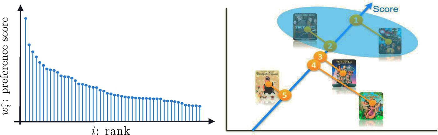
Figure 11.13: One way to rank top K items is to first estimate the latent scores {w*i}ni=1 and then rank them (left panel). This yields the actual rank of items (right panel)
To accomplish the above complicated task, we need a statistical model. We assume that there is a positive latent score w7 that is associated with item i so that
 (11.47)
for any pairs (i, j). Such a model is referred to as the Bradley-Terry-Luce model (Bradley and Terry, 1952; Luce, 1959). Thus, our task is to get an estimate of the latent score vector w* = (w*1, …, w*n)T so that we can rank the items according to the preference scores. The idea is depicted in Figure 11.13. Note that w* can only be identified up to a constant multiple so that we will assume that it is a probability vector. Hunter (2004) discussed an MM algorithm for fitting the Bradley-Terry-Luce model.
We do not assume that we have all pairwise comparisons available. In fact, there are only a small fraction of pairs that have ever competed. The pairwise comparisons form a graph G, in which items are vertices and edges indicate whether the two items have been compared. See Figure 11.14. Let ε be the edge set of the graph G. For two items (i, j) ∈ ε, we have obtained Lij
independent comparisons:
 (11.48)
Let p̂ij be the proportion that the jth item beats the ith one. For theoretical studies, we may assume that G is a realization of the Erdös-Rényi graph.
Figure 11.14: Comparison graph for top K ranking. Each pair in the graph has matched Lij times, with proportion p̂ij that the ith item beats the ith item.
A simple and naive ranking is to compute the overall proportion p̂i of winning that item i has ever competed. Then, rank the items according to {p̂i}nj=1This method ignores the ranks of the competitors item i compared with. With a probabilistic model, a natural method is the maximum likelihood method. Conditioning on G, the likelihood of the observed data is the product of those of Bernoulli’s:
The log-likelihood is given by
 (11.49)
Parametrizing θi log wi yields a logistic type of regression and the log-likelihood function is convex. To stabilize the high-dimensional likelihood, one can also regularize the likelihood function by using

which is given by
 (11.50)
Now, let us consider the spectral method, which is also referred to as rank centrality. Without loss of generality, we assume that w* has been normalized to a probability vector. The idea is to create a Markov chain on the graph G such that w* is its invariant distribution, also called stationary distribution. Let us define the transition matrix P* as
 (11.51)
where ε is the set of edges of the graph G and d is a parameter. When d is sufficiently large (e.g. the maximum of the degrees) so that the diagonal entries are non-negative, the matrix P* is a transition probability matrix: each row has a sum equals to 1. This Markov chain prefers to walk to the state with a higher score. It is easy to verify that P is a transition matrix with the detailed balance

Therefore,
or put in the matrix notation
 (11.52)
In other words, w* is the leading left eigenvector of P* with eigenvalue 1. It is also the stationary distribution of the Markov chain with transition matrix P*.
The spectral method replaces the unknown transition matrix by its empirical counterpart P̂, whose (i, j) element is given by
 (11.53)
If d > dmax, the maximum degree of the graph, then P̂ is a transition matrix (Exercise 11.13). In practice, we take d = 2dmax.
Negahban, Oh and Shah (2017) establish the L2-rate of convergence for the spectral estimator ŵ. Chen, Fan, Ma, and Wang (2019) improve their results and establish further the maximum entrywise estimation error. As a result, they were able to obtain the selection consistency for both the spectral method and the regularized MLE. They show that the sampling complexity achieves the information low bound given by Chen and Suh (2015). Additional references can be found in the papers by Negahban, Oh and Shah (2017) and Chen, Fan, Ma, and Wang (2019). In particular, the latter give a comprehensive review on the recent development on this topic (see Section 2.7 there).
Algorithm 11.2 Spectral method for top K-ranking (Rank Centrality)
1. Input the comparison graph G, sufficient statistics {p̂ij, (i, j) ∈ ε}, and the normalization factor d.
2. Define the probability transition matrix P̂ = [P̂i,j]l≤i,j≤n as in (11.53).
3. Compute the leading left eigenvector ŵ of P̂.
4. Output the K items that correspond to the K largest entries of ŵ.
11.4.5 Gaussian mixture models
As an illustration of the applications of spectral methods to nonconvex optimization, let us consider the Gaussian mixture model:
 (11.54)
with unknown parameters {wk, µk, σ2k}Kk=1. The likelihood function based on a random sample {Xi}ni=1 from model (11.54) can easily be found (Exercise 11.14), but the function is non-convex, which imposes computational challenges to find the MLE.
PCA allows us to find a good initial value for the nonconvex optimization problem. Indeed, the classical result of Bickel (1975) shows that for finite dimensional parametric problems, if we start from a root-n consistent estimator, the one-step Newton-Raphson estimator will be statistically efficient. In other words, optimization errors (the distance to a global optimum) will be of smaller order than statistical errors (standard deviations of estimators). Further iterations will only improve the optimization errors, as is more precisely stated in Robison (1988).
The method of moments is very simple in finding root-n consistent estimators. For the mixture model (11.54), the first two moments (Exercise 11.15) are given by
 (11.55)
where ⨂ denote the Kronecker product and the weighted average variances. Therefore, the column space spanned by {µk}pk=1 is the same as the eigen-space spanned by the top K principal components, and σ2w is the minimum eigenvalue of E [X ⨂ X].
To further determine rotation, Hsu and Kakade (2013) introduce the third order tensor method. Suppose that {µk}Kk=1 are linearly independent and wk > 0 for all k ∈ [K] so that the problem does not degenerate. Then σ2w is the minimum eigenvalue of Σ = cov(X); this will be shown at the end of this section. Let v be any eigenvector of Σ that is associated with the eigenvalue σ2w as shown at the end of this section. Define the following quantities:
where we use the notation
and ej is the unit vector with jth position 1. Then Hsu and Kakade (2013) show that
 (11.56)
With {Mi}i=1 replaced by their empirical versions, the remaining task is to solve for all the parameters of interest via (11.56). Hsu and Kakade (2013) and Anandkumar, Ge, Hsu, Kakade and Telgarsky (2014) propose a fast method called the robust tensor power method to compute the estimators. The idea is to orthogonalize {µk} in M3 by using the matrix M2 so that the power method can be used in computing the tensor decomposition.
Let M2 = UDUT be the spectral decomposition of M2, where D is the K × K non-vanishing eigenvalues of M2. Set
 (11.57)
Note that W is really a generalized inverse of M21/2. Then, WTM2W = IK, which implies by (11.56) that
Thus, {µ̃k}Kk=1 are orthonormal and
 (11.58)
Note that the quadratic form WTM2W can be denoted as M2(W, W), which is defined as
where a⨂2 = a ⨂ a. We can define similarly
 (11.59)
where a⨂ = a ⨂ a ⨂ a. Therefore, M3 admits an orthogonal tensor decomposition that is similar to the spectral decomposition for a symmetric matrix and the decomposition can be rapidly computed by the power method. It then can be verified that
 (11.60)
which is merely a rotated version of (11.56).
The idea of estimation is now very clear. First of all, using the method of moments, we get an estimator of M̂3 by (11.60). Using the tensor power method (Anandkumar et al., 2014), we find estimators for the orthogonal tensor decomposition {µ̃k} and its associated eigenvalue {1/√wk}K1=1 in (11.59). The good piece of the news is that we operate in the K-dimensional rather than the original p-dimensional space. We omit the details. Using (11.57) and (11.58), we can get an estimator for µk. We summarize the idea in Algorithm 11.3.
Note that in Algorithm 11.3, the sample covariance can be replaced by the empirical second moment matrix . To see this, by (11.55) and (11.56),

Thus, the top K eigenvalues are {d1 + σ2w,…, dK + σ2w} and the remaining (p – K) eigenvalues are σ2w. The top K eigenvectors are in the linear span of {µk}Kk=1. Let v be an eigenvector that corresponds to the minimum eigenvalue of E[X ⨂ X]. Then, µTkv = 0 for all k ∈ [K] Using the population covariance
we have
Algorithm 11.3 The tensor power method for estimating parameters in the normal mixtures
1. Calculate the sample covariance matrix, its minimum eigenvalue σ̂2w and its associated eigenvector v̂.
2. Derive the estimators M̂1 and M̂2 by using the empirical moments of X, v̂ and σ̂2w.
3. Calculate the spectral decomposition M̂2 = ÛD̂ÛT. Let Ŵ = ÛD̂−1/2. Construct an estimator of M̃3, denoted by M̂3, based on (11.60) by substituting the empirical moments of ŴTX, Ŵ and M̂1. Apply the robust tensor power method in Anandkumar et al. (2014) to M̂3 and obtain {µ̂̃k}Kk=1 and {ŵk}Kk=1.
4. Compute Solve the linear equations M̂1=
Therefore, σ2w is an eigenvalue and v is an eigenvector Σ. We can show further σ2w is indeed the minimum eigenvalue.
The above gives us an idea of how the spectral methods can be used to obtain an initial estimator. Anandkumar et al. (2014) used tensor methods to solve a number of statistical machine learning problems. In addition to the aforementioned mixtures of spherical Gaussians with heterogeneous variances, they include hidden Markov models and latent Dirichlet allocation. Sedghi, Janzamin and Anandkumar (2016) apply tensor methods to learning mixtures of generalized linear models.
11.5 Bibliographical Notes
There is a huge literature on controlling false discoveries for independent test statistics. After the seminal work of Benjamini and Hochberg (1995) on controlling false discovery rates (FDR), the field of large-scale multiple testing received a lot of attention. Important work in this area includes Storey (2002); Genovese and Wasserman (2004), Lehmann and Romano(2005), Lehmann, Romano and Shaffer (2005), among others. The estimation of the proportion of nulls has been studied by, for example, Storey (2002), Langaas and Lindqvist (2005), Meinshausen and Rice (2006), Jin and Cai (2007) and Jin (2008), among others.
Although Benjamini and Yekutieli (2001), Sarkar (2002), Storey, Taylor and Siegmund (2004), Clarke and Hall (2009), Blanchard and Roquain(2009) and Liu and Shao (2014) showed that the Benjamini and Hochberg and its related procedures continue to provide valid control of FDR under positive regression dependence on subsets or weak dependence, they will still suffer from efficiency loss without considering the actual dependence information. Efron (2007, 2010) pioneered the work in the field and noted that correlation must be accounted for in deciding which null hypotheses are significant because the accuracy of FDR techniques will be compromised in high correlation situations. Leek and Storey (2008), Friguet, Kloareg and Causeur (2009), Fan, Han and Gu(2012), Desai and Storey (2012) and Fan and Han (2017) proposed different methods to control FDR or FDP under factor dependence models. Other related studies on controlling FDR under dependence include Owen (2005), Sun and Cai (2009), Schwartzman and Lin (2011), Wang, Zhao, Hastie and Owen (2017), among others.
There is a surge of interest in community detection in statistical machine learning literature. We only brief mention some of these. Since the introduction of stochastic block models by Holland, Laskey and Leinhardt (1983), there have been various extensions of this model. See Abbe (2018) for an overview. In addition to the references in Section 11.4.1, Bickel and Chen (2009) gave a nonparametric view of network models. Other related work on nonparametric estimation of graphons includes Wolfe and Olhede (2013), Olhede and Wolfe (2014), Gao, Lu and Zhou (2015). Bickel, Chen and Levina (2011) employed the method of moments. Amini et al. (2013) studied pseudo-likelihood methods for network models. Rohe, Chatterjee and Yu (2011) and Lei and Rinaldo (2015) investigated the properties of spectral clustering for the stochastic block model. Zhao, Levina and Zhu (2012) established consistency of community detection under degree-corrected stochastic block models. Jin (2015) proposed fast community detection by score and Jin, Ke and Luo (2017) proposed a simplex hunting approach. Abbe, Bandeira and Hall (2016) investigated the exact recovery problem. Inferences on network models have been studied by Bickel and Sarkar (2016) and Lei (2016), Fan, Fan, Han and Lv(2019a,b).
There has been a surge of interest in the matrix completion problem over the last decade. Candés and Recht (2009) and Recht (2011) studied the exact recovery via convex optimization. Candés and Plan (2010) investigated matrix completion with noisy data. Candés and Tao (2010) studied the optimality of the matrix completion. Cai, Candés and Shen (2010) proposed a singular value thresholding algorithm for matrix completion. Keshavan, Montanari and Oh(2010) investigated the sampling complexity of matrix completion. Eriksson, Balzano and Nowak (2011) studied high-rank matrix completion. Negahban and Wainwright (2011, 2012) derived the statistical error of the penalized M-estimator and showed that it is optimal up to logarithmic factors. Fan, Wang and Zhu (2016) proposed a robust procedure for low-rank matrix recovery, including the matrix completion as a specific example. Cai, Cai and Zhang (2016) and Fan and Kim (2019) applied structured matrix completion to genomic data integration and volatility matrix estimation for high-frequency financial data.
11.6 Exercises
11.1 Suppose that we have linear model Y = XTβ*+ ε with X following model (11.1). Here, we use β* to indicate the true parameter of the model. Consider the least squares solution to the problem (11.3) without constraints:
Let α0, β0, and γ0 be the solution. Show that under condition (11.4), the solution to the above least-squares problem is obtained at

11.2 Suppose that the population parameter β* is the unique solution to E∇L(Y,XTβ)X = 0 where  Let W = (1, uT, fT)T and assume that E∇L(Y, WTθ)W = 0 has a unique solution. Then, under condition (11.9), the unconstrained minimization to the population problem E L(Y, α + uTβ + fTγ) has a unique solution (11.8).
11.3 Let us consider the macroeconomic time series in the Federal Reserve Bank of St. Louisz
http://research.stlouisfed.org/econ/mccracken/sel/
from January 1963 to December of the last year. Let us take the unemployment rate as the Y variable and the remaining as X variables. Use FarmSelect and rolling windows of the past 120, 180, and 240 months to predict the monthly change of unemployment rates. Compute the out-of-sample R2 and produce a table that is similar to Table 11.1. Also report the top 10 most frequently selected variables by FarmSelect in the rolling windows. Note that several variables such as “Industrial Production Index”, “Real Personal Consumption”, “Real M2 Money Stock”, “Consumer Price Index”, “S&P 500 index”, etc, are non-stationary and they are better replaced by computing log-returns: namely the difference of the logarithm of time series.
11.4 Let us dichotomize the monthly changes of unemployment rate as 0 and 1, depending upon whether the changes are non-negative or positive. Run the similar analysis, using FarmSelect for logistic regression, as the previous exercise and report the percent of correct prediction using rolling windows of the past 120, 180, and 240 months. Report also the top 10 variables selected most frequently by FarmSelect in the rolling windows.
11.5 As a generalization of Example 11.1, we consider the one-factor model

Consider again the sample average test statistics Zj = √nX̄.j for the testing problem (11.11). Show that under some mild conditions,

11.6 Analyze the neuroblastoma data again and reproduce the results in Section 11.2.5 using FarmTest and other functions in the R software package. Produce in particular
(a) the scree plots and the number of factors selected in both positive and negative groups;
(b) the correlation coefficient matrix (similar plot to Figure 11.9) for the last 100 genes before and after factor adjustments;
(c) the top 30 significant genes with and without factor adjustments.
11.7 Prove (11.29) and (11.30).
11.8 Use the data in Exercise 11.3 and run principal component regression and augmented principal component regression to forecast the changes of unemployment rates using a rolling windows of 120 months, 180 months, and 240 months, and report the out-of-sample R2 results similar to the PCA block in Table 11.3.
11.9 Let us verify (11.36) using a specific example with three communities.
(a) Assume that communities 1, 2 and 3 consist of nodes {1, …, m}, {m + 1, …, 2m}, and {2m + 1, …, 3m}. Verify (11.36)
(b) Show that the column space of Γ is the eigen-space spanned by the top 3 eigen-vectors of the matrix E A, if P is not degenerate.
(c) Verify the eigenvalues and eigenvectors given in Example 11.3
11.10 For the Erdös-Rényi graph G(n, p),
(a) What is the probability that a node is isolated?
(b) What is the limit of the probability as n → ∞ if p = c/n.
(c) Show that the graph has no isolated node with probability tending to one if p = c(log n)/n for c > 1.
11.11 Simulate a data set from the model given in Exercise 9 with n = 150 (m = 50), diagonal elements of P matrix p = 5(log n)/n, and off-diagonal elements q = p/10. Give the resulting graph, the scree plot of absolute eigenvalues of the adjacency matrix, and the results of spectral analysis using R function kmeans.
11.12 Following the notation in Section 11.4.3, let Zij = XijI(i,j)∈Ω/p. Show that E Zij = E Xij = θij under the Bernoulli sampling scheme.
11.13 Show that the matrix (11.53) is a transition matrix if d > dmax.
11.14 Suppose that we have a random sample {Xi}ni=1 from the Gaussian mixture model (11.54).
(a) Write down the likelihood function.
(b) Simulate a random sample of size n = 1000 from the model (11.54) with p = 1, K = 3, σk = 1 and wk = 1/3 for all k, and µ1 = −1, µ2 = 1 and µ3 = 10. Plot the resulting likelihood function as a function of (μ1, μ2) and a function of (μ2, μ3). Are they convex?
11.15 Prove (11.55).