Chapter 10

Covariance Learning and Factor Models

 

 

 

 

 

High-dimensional measurements are often strongly dependent, as they usually measure similar quantities under similar environments. Returns of financial assets are strongly correlated due to market conditions. Gene expressions are frequently stimulated by cytokines or regulated by biological processes. Factor models are frequently used to model the dependence among high-dimensional measurements. They also induce a low-rank plus sparse covariance structure among the measured variables, which are referred to as factor-driven covariance and idiosyncratic covariance, respectively.

This chapter introduces the theory and methods for estimating a high-dimensional covariance matrix under factor models. The theory and methods for estimating both the covariance matrices and the idiosyncratic covariance will be presented. We will also show how to estimate the latent factors and their associated factor loadings and how well they can be estimated. The methodology is summarized in Section 10.2, where any robust covariance inputs can be utilized and the methods for choosing the number of factors are also presented. Principal component analysis plays a critical role in unveiling latent factors as well as estimating a structured covariance matrix. We will defer the applications of factor models to variable selection, large-scale inferences, prediction, as well as other statistical machine learning problems to Chapter 11.

10.1 Principal Component Analysis

Principal component analysis (PCA) is a popular data processing and dimension reduction technique. It has been widely used to extract latent factors for high dimensional statistical learning and inferences. Other applications include handwritten zip code classification (Hastie, Tibshirani and Friedman, 2009), human face recognition (Hancock, Burton and Bruce, 1996), gene expression data analysis (Misra et al. 2002, Hastie et al. 2000), to name a few.

10.1.1 Introduction to PCA

PCA can be mathematically described as a set of orthogonal linear transformations of the original variables X such that the transformed variables have the greatest variance. Imagine that we have p measurements on an individual’s ability and we wish to combine these measurements linearly into an overall score Z₁ = Σ_j^p ₌₁ξ_1jjX_j = ξ₁^T X. We wish such a combination to differentiate as much as possible individual abilities, namely makes the individual scores vary as large as possible subject to the normalization ‖ξ‖=1. This leads to choosing ξ₁ to maximize the variance of Z₁, i.e.,

Now suppose that we wish to find another metric (a linear combination of the measurements), whose information is unrelated to what we already have, Z₁ that summarizes other aspects of the individual’s ability. It is again to find the linear combination to maximize the variance subject to the normalization and uncorrelatedness constraint. In general, the principal components can be defined sequentially. Given the first k principal components Z_l= ξ_l^T X for 1 ≤ l ≤ k, the (k+1) th principal component is defined as Z_k+1 = ξ_k+1^T X with

(10.1)

In other words, it is defined as the projection direction that maximizes the variance subject to the orthogonality constraints. Note that the sign of principal components can not be determined as ±ξ_k+1 are both the solutions to (10.1). It will soon be seen that the orthogonality constraints here are equivalent to the uncorrelatedness constraints. Figure 10.1 illustrates the two principal components based on the sample covariance of a random sample depicted in the figure.

Assume that Σ has distinct eigenvalues. Then, ξ₁ is the first eigenvector of Σ and _Al is the variance of λ₁. By induction, it is easy to see that the kth principal component ξ_k is the kth eigenvector of Σ. Therefore, PCA can be found via spectral decomposition of the covariance matrix Σ:

(10.2)

where Γ = (ξ₁, …,ξ_p) and Λ = diag(λ₁, • • •, λ_p). Then, the kth principal component is given by Z_k= ξ_k^T X, in which ξ_k will be called the loadings of Z_k. Note that

Hence, the orthogonality constraints and uncorrelatedness constraints are equivalent.

In practice, one replaces Σ by an estimate such as the sample covariance matrix. As an example, let us use the sample covariance matrix S= n^-1 X̃X̃^T where X̃ is the n × p data matrix whose column means have been removed. One may replace n⁻¹ by (n — 1)−¹ to achieve an unbiased estimate of Σ, but it does not matter in PCA. Do the singular value decomposition (SVD) for the data matrix X̃

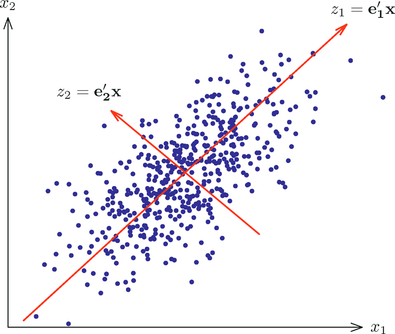
Figure 10.1: An illustration of PCA on a simulated dataset with two variables. z₁ is the first principal component and z₂ is the second one.

where D is a diagonal matrix with elements d₁, …, d_p in a descending order, and U and V are is n × p and p × p orthonormal matrices, respectively. Then,

Hence, the columns of V are the eigenvectors of S. Let v_k be its k^th column. The k^th (estimated) principal component z_k= v^t_kX with realizations {z_k,_i = v_k^Tx_i}iⁿ_{= 1}. Put this as a vector z_k. By XV = UD, we have z_k = d_ku_k, where u_k is the kth column of U.

10.1.2 Power method

In addition to computing the PCA by the SVD, the power method (also known as power iteration) is very simple to use. Given a diagonalizable matrix Σ in (10.2), its leading eigenvector can be computed iteratively via

(10.3)

It requires that the initial value ξ₁⁽⁰⁾ is not orthogonal to the true eigenvector ξ₁. Note that

by using (10.2). Thus, the power suppresses smaller eigenvalues to zero with geometric convergence rate (λ₂/λ₁)^t. Power iteration is a very simple algorithm, but it may converge slowly if λ₂≈ λ₁. With the computed eigenvector, its corresponding eigenvalue can be computed by using λ₁=ξ₁^TΣξ₁.

Now the second eigenvector can be computed by applying the power method to the matrix Σ−λ₁=ξ₁ξ₁^T_.. It is easy to see from (10.2), ξ₂ will be correctly computed so long as λ₃/λ₂ < 1. In general, after computing the first k eigenvalues and eigenvectors, we apply the power method to the matrix

to obtain ξ_k+1. After that, the eigenvalue λ_k+₁ can be computed via λ_k+₁ ξ_k+1^TΣξ_k+1.

10.2 Factor Models and Structured Covariance Learning

Sparse covariance matrix assumption is not reasonable in many applications. For example, financial returns depend on common equity market risks; housing prices depend on economic health and locality; gene expressions can be stimulated by cytokines; fMRI data can have local correlation among their measurements. Due to the presence of common factors, it is unrealistic to assume that many outcomes are weakly correlated: in fact, the covariance matrix is dense due to the presence of the common factor (see Example 10.2 below). A natural extension is the conditional sparsity, namely, conditioning on the common factors, the covariance matrix of the outcome variables is sparse. This induces a factor model.

The factor model is one of the most useful tools for understanding the common dependence among multivariate outputs. It has broad applications in statistics, finance, economics, psychology, sociology, genomics, and computational biology, among others, where the dependence among multivariate measurements is strong. The following gives a formal definition. Recall the notation [p] ={1, … ,p} for the index set.

Definition 10.1 Suppose that we have p-dimensional vector X of measurements, whose dependence is driven by K factors f. The factor model assumes

(10.4)

for each component j =1, …, p. Here, u is the idiosyncratic component that is uncorrelated with the common factors f, B = (b₁, …, b_p)^T are the p × K factor loading matrix with b_ik indicating how much the jth outcome X_j depends on the k^th factor f_k, and a is an intercept term. When Σ_u Var(u) is diagonal, it is referred to as a strict factor model; when Σ_u is sparse, it is called an approximate factor model.

The factor model induces a covariance structure for Σ= Var(X):

(10.5)

It is frequently assumed that Σ_u is sparse, since common dependence has already been taken out. This condition is referred to as the conditional sparsity at the beginning of this section. It is indeed the case when f and u are independent so that Σ_u is the conditional variance of X given f.

10.2.1 Factor model and high-dimensional PCA

Suppose that we have observed n data points {X_i}_i=1ⁿ from the factor model (10.4):

(10.6)

for each variable j =1, … ,p. In many applications, the realized factors {f_i}₌₁ⁿ are unknown and we need to learn them from the data. Intuitively, the larger the p, the better we can learn about the common factors {f_i}. However, the loading matrix and the latent factors are not identifiable as we can write the model (10.6) as

for any invertible matrix H. Thus, we can take H to make Var(H⁻¹f_i)= I_p. There are many such matrices H and we can even take the one such that the columns of (BH) are orthogonal. In addition, E X a + B E f. Therefore, a and E f can not be identified and to make them identifiable, we assume E f =0 so that a =E X. This leads to the identifiability condition as follows.

Identifiability Condition: B^TB is diagonal, Ef =0 and cov(f)= I_p.

Under the identifiability condition, we have the covariance structure

(10.7)

This matrix admits a low-rank + sparse structure, with the first matrix being of rank K. This leads naturally to the following penalized least-squares problem: minimize with respect to Θ and Γ

(10.8)

where S is the sample covariance matrix and ‖ Θ ‖ _* is the nuclear norm (Definition 9.2) that encourages the low-rankness and the second penalty encourages sparseness of Γ = (γ_ij). The above formulation is also known as Robust PCA (Wright et al., 2009; Candés et al., 2011).

How can we differentiate the low-rank and sparse components? The analogy is that real numbers can be uniquely decomposed into integers + fractions. The separation between the first and the second part in (10.7) is the spikeness of the eigenvalues (Wright, et al., 2009; Candés et al., 2011; Agarwal, Negahban, and Wainwright 2012; Fan, Liao and Mincheva, 2013). It is assumed that the smallest non-zero eigenvalues for BB^T are much bigger than the largest eigenvalue of Σ_u so that the eigenspace spanned by the nonzero eigenvalues of BB^T, which is the same as that spanned by the column space of B, can be identified approximately as those of Σ. This leads to the following condition. Let Ω(1) denote a quantity that is bounded away from 0 and ∞.

Pervasiveness assumption: The first K eigenvalues of BB^T have order Ω(p), whereas ‖Σ_u‖₂ =O(1).

This condition is not the weakest possible (see Onatski, 2012), but is often imposed for convenience. It implies that the common factors affect a large fraction of the measurements in X. If the factor loadings {b_j}_j=1^p are regarded as a realization from a non-degenerative K-dimensional population, then by the law of large numbers, we have

which has non-vanishing eigenvalues. Thus, by the Weyl theorem (Proposition 9.2), the eigenvalues of B^TB are of order p and so are the non-vanishing eigenvalues of BB^T, as they are the same. The second condition in the pervasive assumption fulfills easily by the sparsity condition; see the equation just before ((9.16).

Note that the non-vanishing eigenvalues of BB^T and their associated eigenvectors are

(10.9)

where b_j is the j^th column of B, ordered decreasingly in ‖bi‖(Exercise 10.1). Applying Weyl’s theorem and the Davis-Kahan sin θ theorem (Proposition 9.2), we have

Proposition 10.1 Let λ_j = λ_j (Σ) and ξ_j =ξ_j (Σ). Under the identifiability and pervasive condition, we have

Furthermore,

We leave the proof of this proposition as an exercise (Exercise 10.2). The first part shows that the eigenvalues λ_j = Ω(p) for j ≤ K and λ_j = O(1) for j > K. Thus, the eigenvalues are indeed well separated. In addition, the second part shows that the principal component direction ξ_j approximates well the normalized j^th column of the matrix B, for j ≤ K. In other words

(10.10)

for j ≤ K, where we used

In addition, by (10.6) and the orthogonality of matrix B, we have

The last component is the weighted average of weakly correlated noises and is often negligible. Therefore, by using (10.10), we have

(see Exercise 10.3) or in the matrix notation, by using (10.10),

(10.11)

where a =EX can be estimated by, for example, the sample mean. This demonstrates that factor models and PCA are approximately the same for high-dimensional problems with the pervasiveness assumption, though such a connection is much weaker for the finite dimensional problem (Jolliffe, 1986).

Example 10.1 Consider the specific example in which observed random vector X has the covariance matrix Σ= (1 — ρ²)I_p+ ρ²11^T. This is an equicorrelation matrix. It can be decomposed as

In this case, the factor-loading b=ρ1. Averaging out both sides, the latent factor f can be estimated through

Applying this to each individual i, we estimate

which has error √1 − ρ²p⁻¹ Σ_j=1^p u_ij = O_p(p^−½). This shows that the realized latent factors can be consistently estimated.

10.2.2 Extracting latent factors and POET

The connections between the principal component analysis and factor analysis in the previous section lead naturally to the following procedure based on the empirical data.

a) Obtain an estimator and μ̂ of Σ and Σ, e.g., the sample mean and covariance matrix or their robust versions.

b) Compute the eigen-decomposition of

(10.12)

Let {λ̂_k }_k=1^K be the top K eigenvalues and { ξ̂}_k=1^K be be their corresponding eigenvectors.

c) Obtain the estimators for the factor loading matrix

(10.13)

and the latent factors

(10.14)

namely, B̂ consists of the top-K rescaled eigenvectors of Σ and f_i is just the rescaled projection of X_i — µ̂ onto the space spanned by the eigenvectors.

d) Obtain a pilot estimator for Σ_u by Σ_u =Σ_u^p=K+1λjξ_j ξ_jj and its regularized estimator Σ_u,λ by using the correlation thresholding estimator ((9.13).

e) Estimate the covariance matrix Σ= Var(X) by

(10.15)

The use of the high-dimensional PCA to estimate latent factors has been studied by a number of authors. In particular, Bai (2003) proves the asymptotic normalities of estimated latent factors, estimated loading matrix and their products. The covariance estimator (10.15) is introduced in Fan, Liao and Mincheva (2013) and is referred to as the Principal Orthogonal ComplEment Thresholding (POET) estimator. They demonstrate that POET is insensitive to the over estimation on the number of factors K.

When a part of the factors is known such as the Fama-French 3-factor models, we can subtract these factors’ effect out by running the regression as in Section 10.3.1 below to obtain the covariance matrix Σ_u of residuals {u_i}_iⁿ₌₁ therein. Now apply the PCA above further to Σu to extract extra latent factors. Note that these extra latent factors are orthogonal (uncorrelated) with the initial factors and augmented the original observed factors.

The above procedure reveals that

Therefore, the sample covariance between the estimated j^th and k^th factor is

where S is the sample covariance matrix defined by ((9.7). It does not depend on the input µ̂. When the sample cov_ariance is used as the initial estimator, these estimated factors {f_ij}_i=1ⁿ and {f_ij}_i=1ⁿ are uncorrelated for j ≠ k with sample variance 1. In general, they should be approximately uncorrelated with the sample variance approximately 1.

In many applications, it is typically assumed that the mean of each variable has been removed so that intercepts a can be set to zero. When the initial covariance matrix is the sample covariance matrix ((9.7), the solution admits the least-s_quares interpretation. From (10.6), it is natural to find B and F = (f₁, fn)^T to minimize

(10.16)

subject to n⁻¹Σ_i=1ⁿ f_if_i^T =I_K and B^TB diagonal (the identifiability condition). For given B, the solution for the least-s_quares problem is

or in the matrix form F̂ = XBD where X is a n × p data matrix and D =diag (B^TB)⁻¹. Substituting it in (10.16), the objective function now becomes

The solution of this problem is the same as the one given in step c) above, namely, {‖b_j‖²}j=1^K are the top K eigenvalues of the sample covariance matrix n⁻¹ X^T X and the columns {b̃_j / ‖b̃_j ‖)_i=1^K are their associated eigenvectors {ξ_j}_j^K₌₁ (Exercise 10.5). This gives a least-s_quares interpretation.

We can derive similarly that for given F, since the colu_mns of the design matrix F are orthonormal, the least-s_quares estimator is B̂=n⁻¹X^TF. Substituting it in, the objective function now becomes

The solution to this problem is that the columns of F̂/ √n are the top K eigenvectors of the n × n matrix XX^T and B̂ = n⁻¹X^TF̂ (Stock and Watson, 2002). This provides an alternative formula for computing B̂ and F̂. It involves computing top K eigenvalues and their associated eigenvectors for a n × n matrix XX^T, instead of a p × p sample covariance matrix X^TX. If p ≫ n, this method is much faster to compute. We summarize the result as the following proposition. We leave the second result as an exercise (Exercise 10.6).

Proposition 10.2 The solution to the least-squares problem (10.16) is

This is an alternative formula for estimating latent factors based on the sample covariance matrix S, namely, it is the same as (10.13) and (10.14) with Σ= S, when X= 0 (the demeaned data).

The advantages of the robust covariance inputs have been demonstrated by Fan, Liu and Wang (2018) and Fan, Wang and Zhong (2019) for different covariance inputs. As an illustration, we simulate data from the factor model with (f_i, u_i) jointly following a multivariate t-distribution with degrees of freedom ν whose covariance matrix is given by diag(I_K, 5I_p) and factor loadings from N(0, I_K). Larger ν corresponds to a lighter tail and ν =∞ corresponds to a multivariate normal distribution. Note that the observed data is generated as X_i= Bf_i + u_i, which requires us to have the matrix B first and then jointly drawing (f_i, u_i) in order to compute X_i. Each row of the loading matrix B is independently sampled from a standard normal distribution. The true covariance is Σ= BB^T + 5I_p in this factor model.

We vary p from 200 to 900 with sample size n= p/2, and fixed number of factors K =3. The thresholding parameter in ((9.13) was set to λ= 2. For data simulated from heavy distribution (ν= 3), moderately heavy distribution (ν=5) 5) and the light distribution (ν= ∞, normal), we compared the performance of the following four methods

(1) the sample covariance;

(2) the adaptive Huber’s robust estimator;

(3) the marginal Kendall’s tau estimator; [marginal estimated variances are taken from (2)]

(4) the spatial Kendall’s tau estimator.

For each method, we compute the estimation errors ‖Σ̂_u^τ − Σ_u‖,‖(Σ̂_u^τ)⁻¹− Σ⁻¹‖and ‖Σ̂^τ − Σ‖_Σ (see the definition after Example 10.2) and report its ratio with respect to method (1), the sample covariance method. The results are depicted in Figure 10.2 based on 100 simulations. For the first two settings, all robust methods outperform the sample covariance; more so for ν= 3. For the third setting (normal distribution), method (1) outperforms, but the price that we pay is relatively small.

10.2.3 Methods for selecting number of factors

In applications, we need to choose the number of factors K before estimating the loading matrix, factors, and so on. The number K can be usually estimated from the eigenvalues of the pilot covariance estimator Σ̂. Classical methods include likelihood ratio tests (Bartlett, 1950), the scree plot (Cattell, 1966), among others. The latter basically examines the percentage of variance explained by the top k eigenvectors, defined as

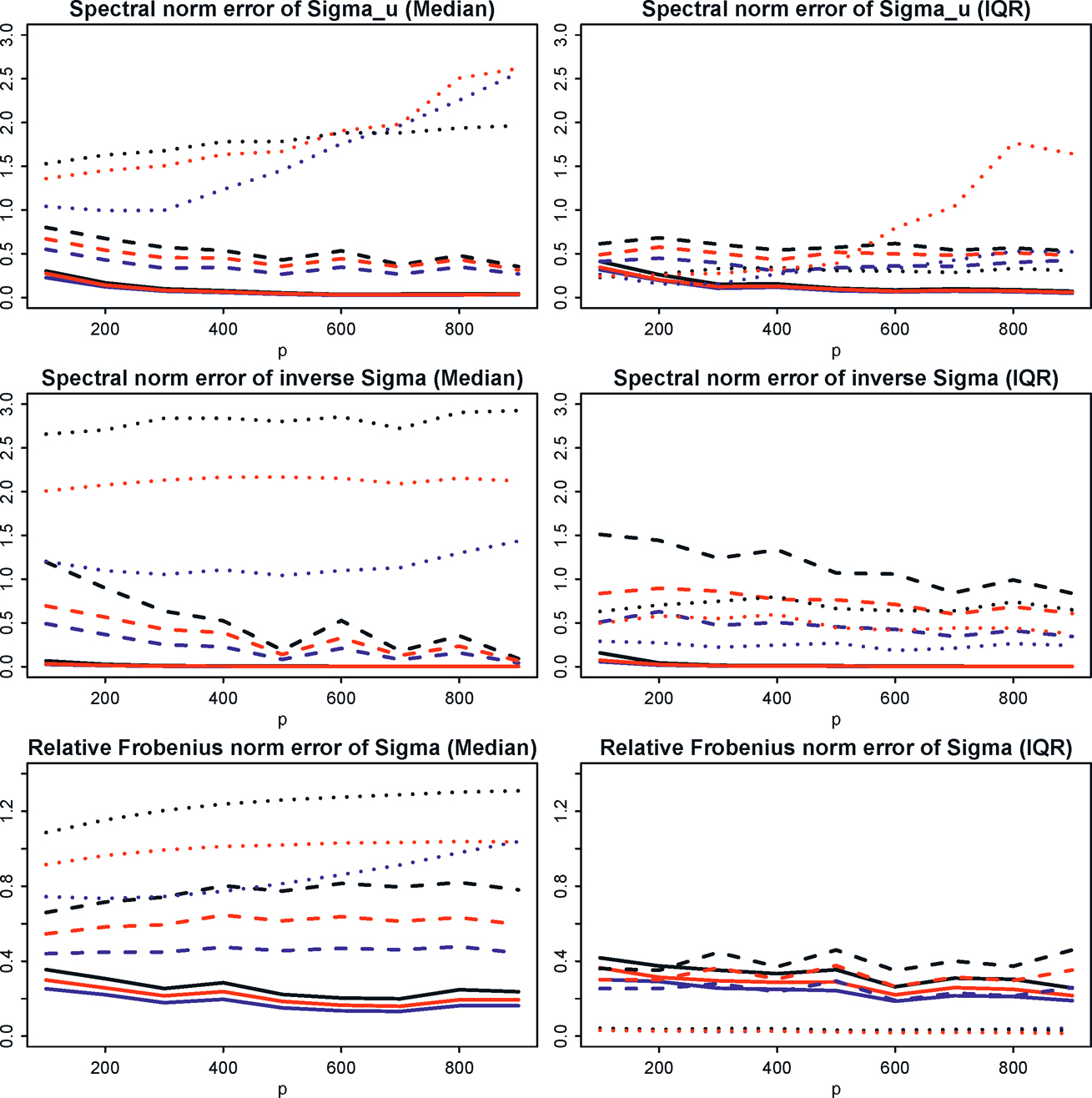
Figure 10.2: Error ratios of robust estimates against varying dimensions. Blue lines represent errors of Method (2) over Method (1) under different norms; black lines errors of Method (3) over Method (1); red lines errors of Method (4) over Method (1). The median errors and their IQR’s (interquartile range) over 100 simulations are reported. Taken from Fan, Wang, Zhong (2019).

One chooses such a k so that p̂_k fails to increase noticeably.

Let R̂ = diag(Σ̂)^−½Σ̂̂ diag(Σ̂̂ )^−½ be the correlation matrix with corresponding eigenvalues (λ_j(R)}. A classical approach is to choose

as the number of factors. See, for example, Guttman (1954) and Johnson and Wichern (2007, page 491). When p is comparable with n, an appropriate modification is the following Adjusted Eigenvalues Thresholding (ACT) estimator by Fan, Guo and Zheng, 2020)

where λ_j^C (R) the bias-corrected estimator of the j^th largest eigenvalue. This is a tuning-free and scale-invariant method. Here, we introduce a few more recent methods: the first one is based on the eigenvalue ratio, the second one based on eigenvalue differences, and the third one based on information criteria. They are in the order of progressive complexity. As noted before, for estimating covariance matrix E, POET estimator Σ_λ is insensitive to the overestimation of K, but is sensitive to the underestimation of K.

For a pre-determined k_max, the eigenvalue ratio estimator is

(10.17)

where k_max is a predetermined parameter. This method was introduced by Luo, Wang, and Tsai (2009), Lam and Yao (2012) and Ahn and Horenstein (2013). Intuitively, when the signal eigenvalues are well separated from the rest of the eigenvalues, the ratio at k =K should be the largest. Under some conditions, the consistency of this estimator, which does not involve tuning parameters, has been established.

Onatski (2010) proposed to use the differences of consecutive eigenvalues. For a given δ > 0 and pre-determined integer k_max, define

Using a result on the empirical distribution of eigenvalues from random matrix theory, Onatski (2010) proved the consistency of K̂₂(δ) under the pervasiveness assumption. The paper also proposed a data-driven way to determine b from the empirical eigenvalue distribution of the sample covariance matrix.

A third possibility is to use an information criterion. Define

where the second equality is well known (Exercise 10.7). For a given k, V(k) is interpreted as the sum of squared residuals, which measures how well k factors fit the data. A natural estimator K₃ is to find the best k ≤ k_max such that the following penalized version of V(k) is minimized (Bai and Ng, 2002):

and σ̂² is any consistent estimate of (np)⁻¹ Σ_i=1ⁿ Σ_j=1^a Eu_ji². Consistency results are established under more general choices of g(n, p).

10.3 Covariance and Precision Learning with Known Factors

In some applications, factors are observable such as the famous Fama- French 3 factors or 5 factors models in finance (Fama and French, 1992, 2015). In this case, the available data are {(f_i, X_i)}_i=1ⁿ and the factor model is really a multivariate linear model (10.6). This model also sheds lights on the accuracy of covariance learning when the factors are unobservable.

In other applications, factors can be partially known. In this case, we can run the regression first to obtain the residuals. Then, apply the methods in Section 10.2.2 to an estimate of the residual covariance matrix. This gives new estimated factors and the regularized estimation of the covariance matrix. They can be further used for prediction and portfolio theory. See Chapter 11.

10.3.1 Factor model with observable factors

Running the multiple regression to the model (10.6), we obtain the least-squares estimator for the regression coefficients in each component:

This yields an estimator of the loading matrix B̂ = (b̂₁^T…, b̂p^T )^T. Let

be the residual of model (10.6). Denote by Σ_u the sample covariance of the residual vectors {û_i}i=1ⁿ.

Since Σ_u is sparse, we can regularize the estimator Σ̂_u by the correlation thresholding ((9.13), resulting in Σ_u,λ. This leads to the regularized estimation of covariance matrix by

(10.18)

where Σ̂_f is the sample covariance matrix of {f_i}_i=1ⁿ. In particular, when λ = 0, Σ_u,λ, = Σ_u, the sample covariance matrix of {û_i}_i=1ⁿ, and Σ̂_λ reduces to the sample covariance matrix of {X_i}i=1ⁿ. When λ=√n/logp, which is equivalent to applying thresholding 1 to the correlation matrix so that off-diagonals are set to zero, Σ̂_u,λ = diag(Σ̂_u), and our estimator becomes

(10.19)

This estimator, proposed and studied in Fan, Fan, Lv (2008), is always positive definite and is suitable for the strict factor model.

Let m_u,_p be the sparsity measure ((9.15) applied to Σ_u and r_n be the uniform rate for the residuals in L₂:

(10.20)

Under some regularity conditions, Fan, Liao and Mincheva (2011) showed that

where The results can be obtained by checking the conditions of pilot estimator Σ_u (see Theorem 9.1). For the sub-Gaussian case, it can be shown that so that the rates are the same as those given in Theorem 9.1.

What are the benefits of using the regularized estimator (10.18) or (10.19)? Compared with the sample covariance matrix, Fan, Fan and Lv (2008) showed that the factor-model based estimator has a better rate for estimating Σ̂⁻¹ and the same rate for estimating Σ. This is also verified by the extensive studies therein. The following simple example, given in Fan, Fan, Lv (2008), sheds some light upon this.

Example 10.2 Consider the specific case K = 1 with the known loading B = 1_p and Σ_u = I_p, where 1_p is a p-dimensional vector with all elements 1. Then Σ = σ_f² 1_p 1_p^′ + I_p, and we only need to estimate σ_f² ≡ Var(f) using, say, the sample variance σ̂_f²=1/n Σ_i=1ⁿ(f_i− f̄)². Then, it follows that

Therefore, by the central limit theorem, <disp-formula> is asymptotically normal. Hence ‖Σ−Σ‖ ₂₌O_p(p/√n) even for such a toy model, which is not consistent when p ≍ √n.

To provide additional insights, the eigenvalues for this toy model are (1 + σ_f²)p, 1, …,1. They are very spiked. The largest eigenvalues can at best be estimated only at the rate O_p(p/√n). On the other hand, Σ⁻¹ has eigenvalues (1 + σ_f²)⁻¹/p, 1, …,1, which are much easier to estimate, turning the spike ones into an easily estimated one.

The above example inspires Fan, Fan and Lv (2008) to consider the relative losses based on the discrepancies between the matrix Σ^−½ Σ̂ Σ^−½ and I_p. Letting ‖A‖_Σ =p^−½‖Σ^−½AΣ^−½ they define the quadratic loss

and the entropy loss (James and Stein, 1961; see also ((9.8))

These two metrics are highly related, but the former is much easier to manipulate mathematically. To see this, let λ₁, …, λ_p be the eigenvalues of the matrix Σ^−½Σ̂ Σ^−½. Then

whereas the entropy loss can be written as

by Taylor expansion at λj = 1. Therefore, they are approximately the same (modulus a constant factor) when Σ is close to Σ.

The discrepancy of Σ^−½Σ̂̂ Σ^−½ and I_p is also related to the relative estimation errors of portfolio risks. Thinking of X as a vector of returns of p assets, w^TX is the return of the portfolio with the allocation vector w, whose portfolio variance is given by Var(w^TX) =ww. The relative estimation error of the portfolio variance is bounded by

another measure of relative matrix estimation error. Note that the absolute error is bounded by

In comparison with the sample covariance, Fan, Fan, Lv (2008) showed that there are substantial gains in estimating quantities that involve Σ⁻¹ using regularized estimator (10.19), whereas there are no gains for estimating the quantities that use Σ directly. Fan, Liao and Mincheva (2011) established the rates of convergence for a regularized estimator (10.18).

10.3.2 Robust initial estimation of covariance matrix

Fan, Wang and Zhong (2019) generalized the theory and methods for robust versions of the covariance estimators when factors are observable. Let Z_i = (X_i^T, f_i^T )^T. Then, its covariance admits the form (Exercise 10.10)

Using the estimator Σ_z we estimate BΣ_fB^T through the identity

and obtain

Note that each element of the p × p matrix Σ₁₂Σ₂₂⁻¹Σ₂₁ involves summation of K² elements and each element is estimated with rate √log p/n. Therefore, we would expect that

Here, we allow K to slowly grow with n. Apply the correlation thresholding ((9.13) to obtain Σ̂_u^τ and produce the final estimator for Σ:

As noted in Remark 9.1, the thresholdling level should now be λω_n√σ̂_u,iiσ̂_u,jj, with aforementioned ω_n.

Theorem 10.1 Suppose that the minimum and largest eigenvalues of Σ_u ∈ C_q (m_p) and Σ_f are bounded from above and below and that ‖B‖is bounded and λ_K(Σ) > cp for some c > 0. If the initial estimator satisfies

(10.21)

and Km_pω_n^1−q→ 0 with ω_n= K²√log p/n, then we have

(10.22)

and

(10.23)

The above results are applicable to the robust covariance estimators in Section 9.3, since they satisfy the elementwise convergence condition (10.21). They are also applicable to the sample covariance matrix, when data Z_i admits sub-Gaussian tails. In particular, when K is bounded, we have ω_n = √log p/n. If, in addition, q = 0, then the rates now become

and

To provide some numerical insights, Fan, Liao and Mincheva (2011) simulate data from a three-factor model, whose parameters are calibrated from the Fama-French model, using the returns of 30 industrial portfolios and 3 Fama-French factors from Jan 1^st, 2009 to Dec 31^st, 2010 (n=500). More specifically,

1. Calculate the least-squares estimator B̂ based on the regression of the returns of the 30 portfolios on the Fama-French factors. Then, compute the sample mean vector μ_B and sample covariance matrix Σ_B of the rows of B. The results are depicted in Table 10.1. We then simulate {b_i}_i=1^p from the trivariate normal N(μ_B, Σ_B).

Table 10.1: Mean and covariance matrix used to generate b

μB		ΣB
1.0641	0.0475	0.0218	0.0488
0.1233	0.0218	0.0945	0.0215
-0.0119	0.0488	0.0215	0.1261

2. For j = 1, • • •, 30, let (3₃ denote the standard deviation of the residuals of the regression fit to the jth portfolio returns, using the Fama-French 3 factors. These standard deviations have mean a = 0.6055 and standard deviations σ_SD = 0.2621 with min(σ̂_j) = 0.3533 and max(σ̂_j) = 1.5222. In the simulation, for each given dimensionality p, we generate σ₁, …,σ_p independently from the Gamma distribution G(α, β), with mean αβ and standard deviation √αβ selected to match σ̄ = 0.6055 and σ_SD = 0.2621. This yields α = 5.6840 and β= 0.1503. Further, we create a loop that only accepts the value of σ_i if it is between [0.3533, 1.5222] to ensure the side constraints. Set D= diag{σ₁², …, σ_p²,}. Simulate a sparse vector s= (s₁, …, s_p)′ by drawing s_i~ N(0,1) with probability 0.2/√p log pand s_i = 0 otherwise. Create a sparse covariance matrix Σ_u=D+ss′—diag{s₁², …, s_p²}. Create a loop to generate Σ_u multiple times until it is positive definite.

3. Compute the sample mean μ_f and sample covariance matrix Σ_f of the observed Fama-French factors and fit the vector autoregressive (VAR(1)) model f=μ +Φf_i-1+ε_i (i∈[500]) the Fama-French 3 factors to obtain 3 × 3 matrix Φ and covariance matrix Σ_ϵ. These fitted values are summarized in Table 10.2. In the simulation, we draw the factors f_i from the VAR(1) model with ε_i‘s drawn independently from N₃(0, Σϵ).

Based on the 200 simulations, Fan, Liao and Mincheva (2011) computed the estimation errors ‖Σ_λ—Σ‖_Σ, ‖Σ_λ-Σ‖_max and ‖Σ_λ-Σ⁻¹‖₂^. The results for the sample covariance are also included for comparison and are depicted in Figure 10.3 for p ranging from 20 to 600.

First of all, the estimation error grows with dimensionality p. The regularized covariance matrix outperforms the sample covariance matrix whenever Σ⁻¹ is involved. In terms of estimating Σ, they are approximately the same.

Table 10.2: Parameters for generating observed factors.

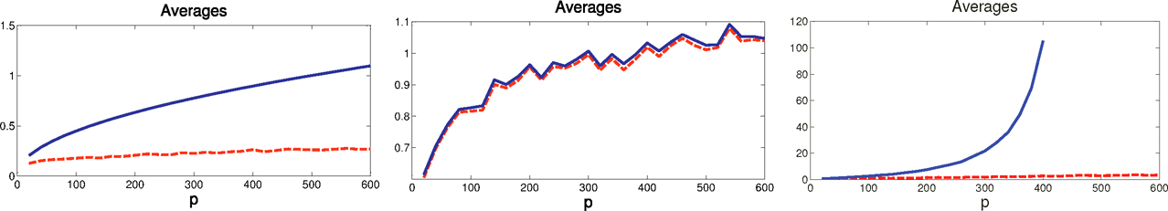
Figure 10.3: The averages of estimation errors ‖Σ_λ —Σ‖_Σ, ‖Σ_λ — Σ‖ _max and ‖Σ̂_λ⁻¹−Σ⁻¹‖₂, based on 200 simulations (red). The results for the sample covariance matrix are also included for comparison (blue). Adapted from Fan, Liao and Mincheva (2011)

This is consistent with the theory and phenomenon observed in Fan, Fan and Lv (2008). For estimating Σ⁻¹, when p is large, the sample covariance gets nearly singular and performs much worse.

10.4 Augmented Factor Models and Projected PCA

So far, we have treated B and f_i as completely unknown and infer them from the data by using PCA. However, in many applications, we do have side information available. For example, the factor loadings of the ^jth stock on the market risk factors should depend on the firm’s attributes such as the size, value, momentum and volatility and we wish to use the augmented information in extracting latent factors and their associated loading matrix. Fan, Liao, and Wang (2016) assumed that factor loadings of the j^th firm can be partially explained by the additional covariate vector W_j and modeled it through the semiparametric model

(10.24)

where g_k(W_j) is the part of factor loading of the j^th firm on the k^th factor that can be explained by its covariates. This is a random-effect model, thinking of coefficients {b_jk} as realizations from model (10.24). Using again the matrix notation (10.6), the observed data can now be expressed as

(10.25)

where the (j, k)^th element of G(W) and Γ are respectively g_k(W_j) and γ_jk.

Similarly, in many applications, we do have some knowledge about the latent factors f_i. For example, while it is not known whether the Fama-French factors W_i are the true factors, they can at least explain a part of the true factors, namely,

(10.26)

Thus, the Fama-French factors are used as the augmented information {W_i}. Using the matrix notation (10.6), the observed data can be expressed as

Using (10.26), assuming u_i is exogenous in the sense that E(u_ilW_i) = 0, we have

(10.27)

This is a noiseless factor model with “new data” X̃_i and common factor f̃_i. The matrix B can be estimated with better precision. Indeed, it can be solved from the equation (10.27) if n ≥ K.

The projected PCA was first introduced by Fan, Liao and Wang (2016) for model (10.25), but it is probably easier to understand for model (10.26), which was considered by Fan, Ke and Liao (2019+). Regress each component of X_i on W_i to obtain the fitted value X̂_i. This can be linear regression or nonparametric additive model (see below) or kernel machine, using the data {(W_i, X_ij)}_i=1ⁿ for each variable X_j, j = 1, … ,p. Run PCA on the projected data {X_i}_i=1ⁿ to obtain an estimate of B and f_i = g(W_i) as shown in (10.27). Denote them by B̂ and ĝ(W_i), respectively. With this more precisely estimated B̂, we can now estimate the latent factor f_i using (10.14) and estimate γ_i by γ̂_i = f_i — ĝ(W_i). We can even compute the percentage of f_i that is explained by W_i as

We now return to model (10.24). It can be expressed as

where g(W_i) and γ_i are the j^th row of G(W) and Γ in (10.25), respectively. Suppose that u_ij is exogenous to W_j. Then, by (10.24), we have

This is again a noiseless factor model with the “new data” X̃_ij and the same latent factor f_i. The regression is now conducted across j, the firms. To see why f_i is not altered in the above operation, let us consider the sample version. Let P be the p × p projection matrix, corresponding to regressing {X_ij}_j^p₌₁ on {_Wj}_j^P₌₁ (see the end of this section for an example of P) for each given i. Now, multiplying P to (10.25), we have

(10.28)

using

(10.29)

This is an approximate noiseless factor model and the latent factors f_i can be better estimated. As noted at the end of Section 10.2.2, F̂√n are the K eigenvectors of the n × n matrix PX(PX)^T =XPX^T and B̂ = n⁻¹X^TF̂ using a better estimated factor F̂.

The above discussion reveals that as long as the projection matrix P can smooth out the noises u_i and {γ_jk}_j^p₌₁, namely, satisfying (10.24), the above method is valid. To see the benefit of projection, Fan, Liao, and Wang (2016) considered the following simple example to illustrate the intuition.

Example 10.3 Consider the specific case where K =1 so that the model (10.24) reduces to

The projection matrix should now be the local averages to estimate g. Assume that g(·) is so smooth that it is in fact a constant β > 0 so that the model is now simplified to

In this case, the local smoothing now becomes the global average over j, which yields

where X_i, γ̄̄ and ū_i are the averages over j. Hence, an estimator for the factor is f̂_i=X̄_i/β̂̂. Using the normalization n⁻¹ Σ_i=1ⁿ f̂_i²=1, we have

Thus, the rate of convergence for f̂_i is O(1/√p), regardless of the sample size n, as X̄_i is the average over p random variables.

We now show how to construct the projection matrix P for model (10.24); similar methods apply to model (10.26). A common model for multivariate function g_k (W_j) is the nonparametric additive model and each function is approximated by a sieve basis, namely,

where L is the number of components in W_i, {ø_k(·)}_m=1^M is the sieve basis (the same for each kl for simplicity of presentation). Thus,

where a_k is the LM-dimensional regression and

Set Φ(W)= (ø(W₁), …, ø(W_p))^T. Then,

is the projection of the matrix of regression of any response variable {Z_j}_j=1^p on {W_j}_j=1^P through the additive sieve basis:

namely the fitted value Ẑ = PZ. See Section 2.5. Clearly, the projection matrix P satisfies (10.29). In our application, Z_j= X_ij(j = 1, …,p) for each fixed i.

In summary, as mentioned before, we extract the latent factors F̂ by taking the top K eigenvectors of the matrix XPX^T multiplied by √nand B̂ = n⁻¹X^TF̂.

10.5 Asymptotic Properties

This section gives some properties for the estimated parameters in the factor model given in Section 10.2.2. In particular, we present the asymptotic properties for the factor loading matrix B, estimated latent factors {f̂_i}_i=1ⁿ, as well as POET estimators Σ̂̂̂λ^τ and Σ̂̂λ. These properties were established by Fan, Liao and Mincheva (2013). We extend it further to cover robust inputs. The asymptotic normalities of these quantities were established by Bai (2003) for the sample covariance matrix as an input, with possible weak serious correlation.

10.5.1 Properties for estimating loading matrix

As in (10.13), B̂ consists of two parts. Let λ̂̃_j = ‖b̃j‖² and ξ_i=b̃̃_j/‖b_j‖. Then, by Proposition 10.1 and the pervasiveness assumption, we have λ̂̃̃_j = Ω(p) if ‖Σu‖ = o(p). Thus, ‖ξ̃̃ ‖_max= Ω (p^−½) as long as ‖B‖max is bounded. In other words, there are no spiked components in the eigenvectors {ξ̃̃_j}j=1^K. By Proposition 10.1 again, there are also no spiked components in the eigenvectors {ξ_j}_j=1^K.

Following Fan, Liu and Wang (2018), we make {λ_j}_j=1^K and {ξ_j}_j=1^K modulus to facilitate the flexibility of various applications. In others, {λ_j}_j=₁^K and {ξ̂ _j}^K_j=1 do not need to be the eigenvalues and their associated eigenvectors of Σ̂. They require only initial pilot estimators Σ̂̂, Λ̂, Γ for covariance matrix Σ, its leading eigenvalues Λ =diag(λ₁, …, λ_K) and their corresponding leading eigenvectors Γ_p×K = (ξ_1,…,ξ_K) to satisfy

(10.30)

These estimators can be constructed separately from different methods or even sources of data. We estimate B̂ as in (10.13) and f_i as in (10.14) with ξ̂_j now denoting the j^th column of Γ̂. We then compute Σ̂_u = Σ̂−Γ̂Λ̂Γ̂^T, and construct the correlation thresholded estimator Σ_u and Σ as in (10.15). Here, we drop the dependence on the constant λ in (10.15) for simplicity and replace the rate √log p/n there by

(10.31)

to reflect the price that needs to be paid for learning the K latent factors. The term 1/√p reflects the bias of approximating factor loadings by PCA (see (10.10)) and the term √log p/n reflects the stochastic error in the estimation of PCA.

Theorem 10.2 Suppose that the top K eigenvalues are distinguished and the pervasiveness condition holds. In addition ‖B‖_max, ‖Σ_u‖ are bounded. If (10.30) holds, then we have

(10.32)

Fan, Liao and Mincheva (2013) showed that for the sample covariance matrix under the sub-Gaussian assumption, condition (10.30) holds even for weakly dependent data. Therefore, the conclusion of Theorem 10.2 holds. Fan, Liu and Wang (2018) proved that condition (10.30) holds for the marginal Kendall’s τ estimator ((9.46) and the spatial Kendall’s τ estimator,

(10.33)

They also showed that (10.30) is also sufficient for the CLIME estimator of the sparse Σ_u⁻¹, which is needed for constructing the sparse graphical model of u. Fan, Wang and Zhong (2019) proved the condition (10.30) holds for the elementwise adaptive Huber estimator in Section 9.3. An ℓ_∞ eigenvector perturbation bound was introduced therein in order to establish the desired result.

10.5.2 Properties for estimating covariance matrices

We now state the properties for estimating Σ_u and Σ. The results here are a slight extension of those in Fan, Liao and Mincheva (2013) and Fan, Liu and Wang (2018).

Theorem 10.3 Under condition of Theorem 10.2, if Σ_u ∈ C_q(m_p), m_pw_n^1−q = o(1) and ‖Σ_u ^−u‖₂=O(1) then we have for estimating Σ_u

(10.34)

and for estimating Σ

(10.35)

Remark 10.1 The condition ‖Σ_u ^−u‖₂=O(1) is used only to establish the third result in (10.34) and the third result in (10.35). It was not used anywhere else. The third term in the second rate in (10.35) is dominated by the second term if K = O(p/m_p). In establishing the second rate in (10.35), we used the bound

so that we can use the third condition in (10.30). This is usually too crude when K depends on n.

When K is finite, Theorem 10.3 shows that in comparison with the case where the factors are observable (Theorem 10.1), we need to pay an additional price of 1/√p for learning the latent factors. This price is negligible when p≫ n log n.

10.5.3 Properties for estimating realized latent factors

We now derive the properties for estimating the latent factor by (10.14).

Theorem 10.4 Under condition of Theorem 10.2, if ‖µ̂ − µ‖ Op (√p log p/n), then we have for estimating the realized latent factors

(10.36)

Note that E‖ X_i – µ‖² = tr(Σ) = O(Kp) as we have K spiked eigenvalues of order O(p) and similarly E‖B^Tu_i‖²= O(pK²) (see (10.54) and (10.55)). Therefore, we expect

(10.37)

if the random variables ‖x_i –µ‖ and ‖B^Tu_i‖ are sub-Gaussian. Consequently,

(10.38)

Corollary 10.1 Under the conditions of Theorem 10.4 and (10.37), we have

provided max_i <n ‖f_i‖ = OP(√K log n).

Proof. It is easy to see that

Using (10.32) and ‖B‖_max = O(1), the first term is of order

by (10.38). The second term is bounded by

Combining the last two terms, the conclusion follows.

10.5.4 Properties for estimating idiosyncratic components

By (10.6), a natural estimator for u_i is

(10.39)

By definition, we have

By Corrollary 10.1, we have

Corollary 10.2 Under the conditions of Corollary 10.1, we have

Note that if we are interested in the L₂-error, the condition max_j≤_n ‖f_j‖ = Op (√K log n) can be dropped. To see this, note that

The second term is further bounded by

Therefore,

This depends only on the average n⁻¹Σ_i=1ⁿ ‖f_i‖², a rather than the maximum. By using Theorems 10.2 and 10.4, we conclude (Exercise 10.11) that

(10.40)

10.6 Technical Proofs

10.6.1 Proof ofTheorem 10.1

We first give two lemmas. The technique in the proof of Lemma 10.1 will be repeatedly used in the proof of Theorem 10.1. Therefore, we furnish a bit more details. Throughout this section, we use ‖ ·‖ to denote ‖ · ‖ ₂.

Lemma 10.1 For any compatible matrices A and B, we have

Further, for any three compatible matrices A, B and C, we have

Proof. Note that for any symmetric matrix D, ‖D‖I — D ≥ 0 and hence

(10.41)

Let τ_n =p‖AB‖_Σ². Then, by (10.41), we have

Now using the property that tr(CD) = tr(DC), we have

using again (10.41). Finally, using (10.41) one more time, we obtain

Similarly, by using tr(ABB^TA^T) = tr(B^TA^TAB) and using (10.41), we obtain

The first conclusion follows by combining the last two results.

To prove the second conclusion, using (10.41), we have

On the other hand, by using (10.41) again,

Shuffling the order of A, B and C in the calculation of trace, we can also get

The result follows from the combination of the above three inequalities.

Lemma 10.2 Let Σ= B^TΣ_fB+Σ_u. Then, under the assumption of Theorem 10.1, we have

Proof. By the Sherman-Morrison-Woodbury formula ((9.6), we have

By multiplying the two terms in the curly bracket, we obtain

where the third inequality follows by multiplying the two terms in the curly bracket out. Therefore, the conclusion follows.

 

Proof of Theorem 10.1. (i) By Theorem 9.1, to establish (10.22), we need to verify the condition ‖Σ_u − Σ_u ‖_max = O_P(ω_n). Since ‖Σ_u − Σ_u ‖_max Op(√log p/n), all sub-blocks Σ₁₁, Σ₁₂ and Σ₂₂ are estimated with the same uniform rate of convergence. Therefore, we need only to verify the rate for estimating Σ₁₂Σ₂₂⁻¹Σ₂₁. Since each element of this p × p matrix involves only summations K² elements, it follows that

(10.42)

This establishes (10.22).

(ii) First rate in (10.23). We next establish the rate for ‖Σ̂^τ −Σ‖_max. First of all

The former is bounded by max λ_ij, which has the same rate as ‖Σ̂^τ −Σ‖_max= Op(ω_n). Thus, ‖Σ̂^τ −Σ‖_max=Op(ω_n). This and (10.42) entail that

(iii) Second rate in (10.23). We next deal with the relative Frobenius norm convergence. Decompose

(10.43)

We bound the four terms one by one.

The last term is the easiest. Using Lemma 10.1 and (10.22), we have

Here we used ‖Σ̂⁻¹‖≤‖Σ̂⁻¹_u‖, which is bounded by assumption. The bound for Δ₁ uses the obvious inequality

(10.44)

and the fact that ‖Σ̂̂₂₂⁻¹‖ and ‖Σ⁻¹‖are O_p(1). By Lemma 10.1, we have

We next bound the second term. Using the definition and the argument as in Lemma 10.1, it is easy to see that

Using (10.44), the first four products are of order O_P(Klogp/n). Recalling that B = Σ₁₂Σ₂₂⁻¹, we have

which is bounded by Lemma 10.2. Hence Δ₂ = Op(√K logp/n).

We next bound Δ₃. Again, using the argument as in Lemma 10.1, we have

The second factor is bounded as shown above and the first factor is

by Lemma 10.1. Namely, Δ₃ = OP(Kp^−1/2√log p/n).

Combining results above, by (10.43), we conclude that

(iv) Third rate in (10.23). We now establish the rate of convergence for ‖(Σ̂^τ)⁻¹−Σ⁻¹‖ By the Sherman-Morrison-Woodbury formula ((9.6), we have

where A = Σ₂₂ + Σ₂₂^TΣ_u⁻¹Σ₂₁ and D = Σ_u⁻¹Σ_12. Denote by the substitution estimators of A and D, A and D respectively. Then, we have the following bound similar to (10.43):

From (10.22), Δ̃₄ = Op(mpω_n^1-q). For the remaining terms, we need to find the rates for ‖D - D‖,‖A⁻¹‖, ‖D‖ and ‖A⁻¹ −A⁻¹‖ separately. Note that

and hence ‖D‖ = O_P(√Kp). By (10.44) and (10.22), we have

In addition, it is not hard to show

Note that

and by Weyl’s inequality,

Therefore, ‖A⁻¹‖ = O_P(p⁻¹) and

implies

and ‖A⁻¹‖ = O_P(p⁻¹). Incorporating the above rates together, we conclude

Combining rates for Δ̃_i,i = 1, 2, 3, 4, we complete the proof.

10.6.2 Proof of Theorem 10.2

To obtain (10.32), we need to bound separately

Recall B = (b̃₁,…,b̃_K) and BB^T=Γ̃Λ̃Γ̃^T, where Λ̃=diag(‖b̃₁‖²,…, ‖b_K‖²) and the j^th column of Γ̃ is b_j/‖b_j‖By assumption (10.30) and Proposition 10.1, we have for some constant c> 0

(10.45)

Furthermore, by Proposition 10.1, we have

(10.46)

As remarked at the beginning of Section 10.5.1, ‖Γ‖_max = O(1/√p). This together with (10.46) and assumption (10.30) entail

(10.47)

By definition, it is easy to verify for any p × K matrix A and q × K matrix B,

Using this and the decomposition

(10.48)

we have

By using assumption (10.30) and (10.47), we have

Similarly, by (10.46) and (10.47), we have

Substituting the rates in (10.46) into the above bound, we have

Combining the rates of Δ₁ and Δ₂, we prove the first rate of (10.32).

Second rate in (10.32). The idea of this part of the proof follows very similarly to that of the first part. For simplicity of notation, let

Recall ξ̂_jdenotes the j^th column of Γ. Then, the j^th column of B− B is

(10.49)

Using the same decomposition as (10.48), we have

Similarly, we have

This proves the second part of (10.32).

10.6.3 Proof of Theorem 10.3

(i) To obtain the rates of convergence in (10.34), by Theorem 9.1, it suffices to prove ‖Σ_u − Σ_u ‖_max = O_P (w_n). According to (10.30) and (10.32), we have

Hence, (10.34) follows by Theorem 9.1.

(ii) First rate in (10.35): Note that

since the order of the adaptive thresholding is chosen to be the same order as w_n. It then follows from Theorem 10.2 that

(iii) Second rate in (10.35): Let

be the spectral decomposition of Σ. Note that

(10.50)

The second term can easily be bounded as, by Lemma 10.1,

(10.51)

where the last inequality follows from Proposition 9.1(3). We now deal with the first term. It is easy to see that

(10.52)

where

We now deal with each of the terms separately. By Lemma 10.1, we have

Using Proposition 9.1(3) and (2), we have

Therefore, by (10.32), we conclude that

By the triangular inequality, Δ_L2 is bounded by

By Lemma 10.1 and Γ₂^TΓ = 0, we have

By Proposition 9.1(2), we have

Therefore,

since ‖Γ −Γ‖_max= O_P(√logp/(np)).

Using similar arguments, by Lemma 10.1, we have

By the sin θ theorem (Proposition 10.1), we have

Hence, Δ_L2⁽²⁾ = O(K^1/2/p³/²). Combining the bounds, we have

By similar analysis, Δ_L3 is dominated by Δ_L1 and Δ_L2. Combining the terms Δ_L1, Δ_L2, Δ_L3 and Δ_s together, we complete the proof for the relative Frobenius norm.

(iv) Third rate in (10.35): We now turn to the analysis of the spectral norm error of the inverse covariance matrix. By the Sherman-Morrison-Woodbury formula ((9.6), we have

where with B̂ = Γ̂Λ̂^½

with Ĵ =B̂^T(Σ̂_u^τ)⁻¹ B̂ and J = B^TΣ_u⁻¹B. The right-hand side can be bounded by the sum of the following five terms:

Note that I_K +Ĵ ≥ λ_min(Σ̂_u⁻¹. Hence,

Thus, the first term is bounded by

where we used the fact that the operator norm of any projection matrix of 1. The second term is bounded by

To bound the third term, note that

The third term is of order

by using ‖B‖ ≤ √Kp‖_max (Proposition 9.1 (2)). Following the same arguments, it is easy to see that T₄= O_P (T₂) and T₅= O_P (T₁).

With the combination of the above results, we conclude that Δ = Op(K²m_pw_n^1−q) and that ‖(Σ̃^τ)⁻¹ − Σ̃^τ‖₂ = O_P(K²m_pw^1−q_n). This completes the proof.

10.6.4 Proof of Theorem 10.4

Let µ = E X_i. First of all, by (10.6),

Let f_i^* = Λ⁻¹B^T(X_i − µ). Then,

We deal with these two terms separately.

Let us deal with the first term. Observe that

(10.53)

By the assumptions and (10.32), we have

and by Theorem 10.2,

Thus, the first term in (10.53) is always demonstrated by the second term. Similarly, by the assumption, the third term is bounded by

Let U_n =n⁻¹ Σ_i=1ⁿ‖X_i−μ̂ ‖. Then, it follows from (10.53) that

Now, let us deal with U_n. Notice that

(10.54)

Therefore, by the law of large numbers, we have

Thus, we conclude that

We now deal with the second term.

Thus, by (10.54), we have

It remains to calculate

(10.55)

Combinations of these two terms yield the desired results.

Inspecting the above proof, the second result holds using basically the same proof. The third result also holds by using identically the same calculation. Here, we note that the maximum is no smaller than average. Therefore, negligible terms in the previous arguments continue to be negligible. This completes the proof.

10.7 Bibliographical Notes

PCA was first proposed by Pearson in 1901 and later by Hotelling in 1933. A popular classical book on PCA is Jolliffe (1986). Hastie and Stuetzle (1989) developed principal curves and principal surfaces. Kernel PCA in a reproducing kernel Hilbert space was discussed in Schölkopf, Smola and Müller (1999). Johnstone and Lu (2009) considered a rank-1 spiked covariance model and showed the standard PCA produces an inconsistent estimate to the leading eigenvector of the true covariance matrix when p/n → c > 0 and the first principal component is not sufficiently spiked. A large amount of literature contributed to the asymptotic analysis of PCA under the ultra-high dimensional regime, including Paul (2007), Johnstone and Lu (2009), Shen, Shen, Zhu and Marron (2016), and Wang and Fan (2017), among others.

High-dimensional factor models have been extensively studied in econometrics and statistics literature. The primary focus of econometrics literature is on estimating latent factors and the factor loading matrix, whereas in statistics literature the focus is on estimating large covariance and precision matrices of observed variables and idiosyncratic components. Stock and Watson (2002a, b) and Boivin and Ng (2006) estimated latent factors and applied them to forecast macroeconomics variables. Bai (2003) derived asymptotic properties for estimated factors, factor loadings, among others, which were extended further to the maximum likelihood estimator in Bai and Li (2012). Onatski (2012) estimated factors under weak factor models. Bai and Liao (2016) investigated the penalized likelihood method for the approximate factor model. Connor and Linton (2007) and Connor, Matthias and Oliver (2012) consider a semiparametric factor model. See also related work by Park, Mammen, Härdle and Borzk (2009).

The dynamic factor model and generalized dynamic model were considered and studied in Molenaar (1985), Forni, Hallin, Lippi, and Reichlin (2000, 2005). As shown in Forni and Lippi (2001), the dynamic factor model does not really impose a restriction on the data-generating process, rather it is a decomposition into the common component and idiosyncratic error. The related literature includes, for example, Forni et al. (2004), Hallin and Lis̃ka (2007, 2011), Forni et al. (2015), and references therein.

The separations between the common factors and idiosyncratic components are carried out by the low-rank plus sparsity decomposition. It corresponds to the identifiability issue of statistical problems. See, for example, Candés and Recht (2009), Wright, Ganesh, Rao, Peng, and Ma (2009), Candés, Li, Ma and Wright (2011), Negahban and Wainwright (2011), Agarwal, Ne-gahban, and Wainwright (2012). Statistical estimation under such a model has been investigated by Fan, Liao and Mincheva (2011, 2013), Cai, Ma and Wu (2013), Koltchinskii, Lounici and Tsybakov (2011), Ma (2013), among others.

10.8 Exercises

10.1 Let B be a p × K matrix, whose columns b̃_j are orthogonal. If {‖b̃_j‖}_j=1^K are ordered in a non-increasing manner, show

for j = 1,… K. What is λ_K+1(B^T B)?

10.2 Prove Proposition 10.1.

10.3 Consider the linear combination b^Tu. Show that

Referring to the notation in (10.10), deduce from this that

which tends to zero if ‖Σ_u‖₁=o(p) (sparse).

10.4 Consider the one-factor model:

Show that

(a) The largest eigenvalue of Σ = Var(X) is (1 +‖b‖²) with the associated eigenvector b/‖b‖.

(b) Let f_i = b^TX_i/‖b‖². If u_i ~ N(0, I_p), show that

10.5 Suppose that Σ̂=Σ_j=1^pλ̂_jξ̂_jξ̂_j. Let B be a p × K matrix and P = B(B^TB)^-1BT be the project matrix into the column space spanned by B.

(a) Show

is minimized at B₀= linear space spanned by ξ̂̂₁, …,ξ̂̂_K.

(b) The minimum value of the above minimization problem is λ_K+1+…+λ_p.

(c) Prove that B̂ (λ̂₁^1/2ξ̂̂̂₁, …, λ̂₁^1/2ξ̂̂̂_K) is a solution to problem (a).

10.6 Show that the solution given in Proposition 10.2 is the same as (10.13) and (10.14) with Σ̂ = Ŝ, when X = 0.

10.7 Prove the following

where S is the sample covariance. Note that you can use the results in Exercise 10.5 to solve this problem.

10.8 Assume that the factor model (10.6) holds. Note that the least-squares solution is to minimize Σ_i=1ⁿ ‖X_i−a−BF_i‖² with respect to a and B with observable factors {f_i}_i=1ⁿ. This is equivalent to the componentwise minimization outlined below (10.6).

(a) For given B, show that the least-squares estimator for a is â = X̄ - Bf̄, where X̄= n⁻¹ Σ_i=1ⁿ X_i and f̄ =n⁻¹Σ_i=1ⁿ f_i.

(b) Show that the least-squares estimator for B is given by
where S_f⁻¹ is the sample covariance matrix of {f_i}_i=1ⁿ.

(c) Show that

10.9 Continuing with the previous problem, assume further that f_i and ui, are independent.

(a) Conditional on {f_i}, show that

(b) Show that the conditional mean-square error

10.10 Let Z = (X^T, f^T)^T, where X follows the factor model (10.6).

(a) Show that the covariance matrix of Z is given by

(b)Prove that the covariance of the idiosyncratic component is given by

(c) If Σ_z is obtained by the sample covariance matrix of the data Z_i = (X_i^T, f_i)^T show that Σ_u =Σ₁₁₋Σ₁₂Σ₂₂Σ₂₁ is the same as the sample covariance matrix of {û_i}_i=1ⁿ, where û_i is the residual vector based on the least-squares fit, as in Exercise 10.15.

10.11 Prove (10.40).

10.12 Let us consider the 128 macroeconomic time series from Jan. 1959 to Dec. 2018, which can be downloaded from the book website. We extract the data from Jan. 1960 to Oct. 2018 (in total 706 months) and remove the feature named “sasdate” and the features with missing entries. We use M to denote the preprocessed data matrix.

(a)Plot the time series of the variable “HWI” (Help-Wanted Index). Given this, can you explain why people usually use a very small fraction of the historical data to train their models for forecasting?

(b) Extract the first 120 months (i.e. the first 120 rows of M

i. For the standardized data, draw a scree plot of the 20 leading eigenval-ues of the sample covariance matrix. Use the eigen-ratio method with k_max =10 to determine the number of factors K. Compare the result with that using the eigenvalue thresholding {j : λ_j(R) > 1 + p/n}. Here, we do not do eigenvalue adjustments to facilitate the implementations for both methods.

ii. Use the package POET to estimate the covariance matrix. Report the maximum and minimum eigenvalues of the estimated matrix. Print the sub-covariance matrix of the first 3 variables.

(c)The column “UNRATE” of M corresponds to monthly changes of the unemployment rate. We will predict the future “UNRATE” using current values of the other macroeconomic variables.

i. Pair each month’s “UNRATE” with the other macroeconomic variables in the previous month (to do so, you need to drop the “UN-RATE” in the first month and other variables in the last month). Let {(X_t,Y_t)}_t=1^N denote the derived pairs of covariates and responses.

ii. We next train the model once a year using the past 120 months’ data and use the model to forecast the next 12 months’ unemployment rates. More precisely, for each month t ∈ {121 + 12m : m 0, 1, … 40}, we want to forecast the next 12 monthly “UNRATE”s {Y_t+Z}Z1₀ based on {X_t+Z}?1₀, using the past 120 months’ data {(X_t−i,Y_t−i)}_i=1¹²⁰ for training. Implement the FarmSelect method by following the steps: standardize the covariates; fit a factor model; fit Lasso on augmented covariates; output the predicted values {Y_t+i^farm }_i=0¹¹ for {Y_t+i}_i=0¹¹. Also, compute the baseline predictions Ȳ_t+i =1/120 Σ_j=1¹²⁰Y_t-j for all i=0,1,…,11.

iii.Report the out-of-sample R² using

(d) Run principal component regression (PCR) with 5 components for the same task as Part (c) and report the out-of-sample R².

(e) Treat {X_i}⁶⁰_i=1 and {X_60+i}_i=1¹²⁰ as independent and identically distributed samples from two distributions and let μ₁, μ₂ denote their expectations. Use the R package FarmTest to test

Print the indices of the rejected hypotheses.