Chapter 9

Covariance Regularization and Graphical Models

 

 

 

Covariance and precision matrix estimation and inference pervade every aspect of statistics and machine learning. They appear in the Fisher’s dis-criminant and optimal portfolio choice, in Gaussian graphical models where edge represents conditional dependence, and in statistical inference such as Hotelling T-test and false discovery rate controls. They have also widely been applied to various disciplines such as economics, finance, genomics, genetics, psychology, and computational social sciences.

Covariance learning, consisting of unknown elements of square order of dimensionality, is ultra-high dimension in nature even when the dimension of data is moderately high. It is necessary to impose some structure assumptions in covariance learning such as sparsity or bandability. Factor models offer another useful approach to covariance learning from high-dimensional data. We can infer the latent factors that drive the dependence of observed variables. These latent factors can then be used to predict the outcome of responses, reducing the dimensionality. They can also be used to adjust the dependence in model selection, achieving better model selection consistency and reducing spurious correlation. They can further be used to adjust the dependence in large scale inference, achieving better false discovery controls and enhancing high statistical power. These applications will be outlined in Chapter 11.

This chapter introduces theory and methods for estimating large covariance and precision matrices. We will also introduce robust covariance inputs to be further regularized. In Chapter 10, we will focus on estimating a covariance matrix induced by factor models. We will show there how to extract latent factors, factor loadings and idiosyncratic components. They will be further applied to high-dimensional statistics and statistical machine learning problems in Chapter 11.

9.1 Basic Facts about Matrices

We here collect some basic facts and introduce some notations. They will be used throughout this chapter.

For a symmetric m x m matrix A, we have its eigen-decomposition as follows

(9.1)

where λ_i is the eigenvalue of A and v_i is its associated eigenvector. For a m x n matrix, it admits the singular value decomposition

(9.2)

where U is an m x m unitary (othornormal) matrix, ∧ is an m x n rectangular diagonal matrix, and V is an n x n unitary matrix. The diagonal entries λ_i of ∧ are called the singular values of A. The columns of U and the columns of V are known as the left-singular vectors and right-singular vectors of A, respectively:

• the left-singular vectors of A are orthonormal eigenvectors of AA^T;

• the right-singular vectors of A are orthonormal eigenvectors of A^TA;

• the non-vanishing singular values of A are the square roots of the non-vanishing eigenvalues of both A^TA and AA^T.

We will assume the singular values are ordered in decreasing order and use λ_i(A) to denote the i^th largest singular value, λ_max(A) = λ₁(A) the largest singular value, and λ_min (A) = λ_m(A) the minimum eigenvalue.

Definition 9.1 A norm of an n x m matrix satisfies

1. ||A||≥ 0 and ||A||= 0 if and only if A = 0;

2. ||αA||= |α|||A||

3. ||A+B|| ≤ ||A||+||B||;

4. IIAB|| ≤ ||A||||B||, if AB is properly defined.

A common method to define a matrix norm is the induced normml: ||A|| — ma_x||x||=1 ||Ax||. In particular, ||A||_p,q = max_||x|p=₁||Ax||q, which satisfies, by definition,

More specifically, when p = g, it becomes the matrix L_p normml:

It includes, as its specific cases,

1. Operator normml: ||A||₂ = λ_max(A^TA)^1/2, which is also written as ||A||_op or simply ||A||;

2. L₁-normml: ||A||₁= max_jΣ^m_i=1 |a_ij|, maximum L₁-norm of columns;

3. L_∞-normml: ||A||∞ = max Σⁿ_i=1, |a_ij|, maximum L₁-norm of rows.

Definition 9.2 The Frobenius norm is defined as

and the nuclear norm is given by

where {λ_i} are singular values defined in (9.2).

Operator norm is hard to manipulate, whereas ||A||_∞, and ||A||₁ are easier. We have the following inequalities.

Proposition 9.1 For any m x n matrix A, we have

1. ||A||₂ ≤ ||A||_∞ ||A||₁ and ||A||_{2 ≤}||A||₁ if A is symmetric.

2. ||A||_max ≤||A||₂ ≤ (mn)^1/2||A||_max, ||A||_max=max_ij|a_ij|

3. ||A||₂ ≤ ||A||_{F ≤} √r||A||_2, r=rank(A);

4. ||A||_F≤||A||_*≤√r||A||_F, r=rank(A)

5. n^-1/2||A||_∞,≤ ||A||_2≤ m^1/2||A||_∞ and m^-1/2 ||A||₁ ≤||A||₂ ≤n^1/2||A||

Here are two basic results about matrix perturbation. For two m x m symmetric matrices A and A, let Â, let λ₁ ≥ ⋯ ≥ λ_m and λ̂ ≥ ⋯ ≥ λ̂ _m be their eigenvalues with associated eigenvectors vi, • • • , v_m and îri, • • • , îr_m, respectively. For two given integers r and s, write d = s — r

and let σ₁ ≥ ⋯ ≥ σ_d be the singular values of V̂^TV. The d principal angles between their column spaces V and V are defined as where {θ_j}^a_i=1, where θ_j = arccos σ_j. Let

be the d x d diagonal matrix. Note that the Frobenius norm of two projection matrices

(9.3)

Proposition 9.2 For two m x m symmetric matrices A and Â, we have

• Weyl Theoremml: λ_min(Â - A) ≤ λ̂_i -λ̂_i ≤ λ̂_max (Â — A). Consequently, |λ̂̂_i-λ_i|≤||Â-A||.

• Davis-Kahan sin θ Theoremml: With λ̂₀ = ∞, λ_m+1 =-∞ and δ= min{|λ̂- λ̂| : λ̂ ∈ [λ̂s, λ̂_r]λ̂̂ ∈ (∞, λ̂̂_8-1] U [λ̂̂_r+1, ∞)} denoting the eigen gap, we have

The result also holds for the operator norm or any other norm that is invariant under an orthogonal transformation.

The above result is due to Davis and Kahan (1970). Specifically, by taking r = s = i, we have

Note that

Combining the last two results, we have

The eigen gap δ involves both sets of eigenvalues. In statistical applications, it typically replaces λ’_is As by its λ’_is using Weyl’s theorem. Yu, Wang and Samworth (2014) give a simple calculation and obtain

(9.4)

and in particular

(9.5)

We conclude this section by introducing Sherman-Morrison-Woodbury Formula and block matrix inversion. If Σ = BΣ_fB^T +Σ_u, then

(9.6)

Let S = A — BD^-1C be the Schur complement of D. Then

9.2 Sparse Covariance Matrix Estimation

To estimate high-dimensional covariance and precision matrices, we need to impose some covariance structure. Conditional sparsity was imposed in Fan, Fan, and Lv (2008) for estimating a high-dimensional covariance matrix and their applications to portfolio selection and risk estimation. This factor model induces a low-rank plus sparse covariance structure (Wright, Ganesh, Rao, Peng, and Ma 2009; Candés, Li, Ma and Wright, 2011), which includes (unconditional) sparsity structure imposed by Bickel and Levina (2008b) as a specific example. Let us begin with the sparse covariance matrix estimation.

9.2.1 Covariance regularization by thresholding and banding

Let us first consider the Gaussian model where we observed data {X_i}ⁿ_i=1 from p-dimensional Gaussian distribution N(μ, Σ). Natural estimators for μ and Σ are the sample mean vector and sample covariance matrix

(9.7)

They are the maximum likelihood estimator when p ≤ n-1. However, the sample covariance is degenerate when p ≥ n. Since we estimate O(p) elements¹, the noise accumulation will make the sample covariance matrix differs substantially from the population one. See Figure 9.1. It shows that the sample covariance matrix is not a good estimator, without any regularization. This is well documented in the random matrix theory (Bai and Silverstein, 2009).

To make the problem estimable in high-dimension, we need to impose a structure on the covariance matrix. The simplest structure is the sparsity of the covariance Σ. This leads to a penalized likelihood method. The log-likelihood for the observed Gaussian data is

Substitution μ by its MLE X̄, expressing (X_i — X̄)Σ^-1(X_i, — X̄)^T as tr(Σ^-1(X_i — X̄)(X_i — X̄)^T) where tr(A) is the trace of a matrix A, we obtain the negative profile log-likelihood

(9.8)

after ignoring the constant term -n/2 log(2π) and dividing the result by —n/2. Thus, the penalized likelihood estimator is to minimize

(9.9)

_______________

¹1,000 × 1,000 matrix involves over half a million elements, whereas 10,000 x 10,000 contains over 50 million elements!

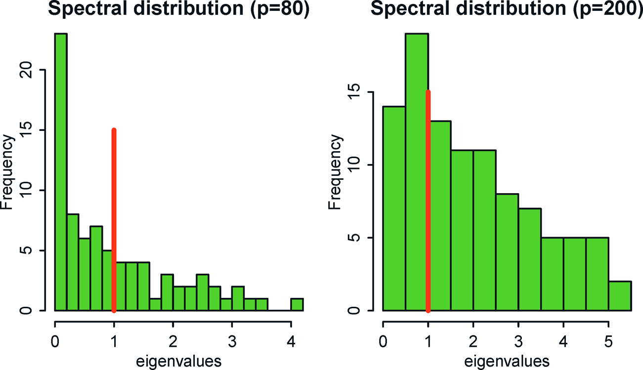
Figure 9.1: Empirical distributions of the eigenvalues of the data {X_i}ⁿ_i=1 simulated from N(0, I_p) for n = 100 and p = 80 (left panel) and p = 200 (right panel). For the case p = 200, there are 100 empirical eigenvalues that are zero, which are not plotted in the figure. Note that the theoretical eigenvalues are 1 for the identity matrix I_p. Theoretical and empirical spectral distributions are very different when n and p are of the same order.

Here, we do not penalize on the diagonal elements, since they are not supposed to be sparse.

The penalized likelihood estimator is unfortunately hard to compute because (9.9) is a non-convex problem even if the penalty function is convex. Bickel and Levina (2008b) explored the sparsity by a simple thresholding operator:

(9.10)

for a given threshold parameter λ, where σ̂_ij =s_ij . In other words, we kill small entries of the sample covariance matrix, whose value is smaller than A. Again, in (9.10), we do not apply the thresholding to the diagonal elements. The thresholding estimator (9.10) can be regarded as a penalized least-squares estimator: Minimize with respect to σ_ij

(9.11)

for the hard thresholding penalty function (3.15). Allowing other penalty functions in Sections 3.2.1 and 3.2.2 leads to generalized thresholding rules (Antoniadis and Fan, 2001; Rothman, Levina and Zhu, 2009).

Definition 9.3 The function τλ,(·) is called a generalized thresholding function, if it satisfies

a) _a) τ_λ(z)| ≤ a|y| for all z, y that satisfy |z — y| ≤ λ/2 and some a > 0;

b) |τ_λ(z) — z| ≤λ, for all z ∈ ℝ

Note that by taking y = 0, we have τ_λ(z) = 0 for |z| ≤ λ/2 and hence it is a thresholding function. It is satisfied for the soft-thresholding function by taking a = 1 and the hard-thresholding function by taking a = 2. It is also satisfied by other penalty functions in Sections 3.2.2.

The simple thresholding (9.10) does not even take the varying scales of the covariance matrix into account. One way to account for this is to threshold on t-type statistics. For example, we can define the adaptive thresholding estimator (Cai and Liu, 2011) as

where SE(σ̂_ij) is the estimated standard error of σ̂_ij.

A simpler method to take the scale into account is to apply thresholding on the correlation matrix (Fan, Liao and Mincheva, 2013). Let ψ̂_λ, be the thresholded correlation matrix with thresholding parameter λ ∈ [0, 1]. Then,

(9.12)

is an estimator of the covariance matrix. In particular, when λ = 0, it is the sample covariance matrix, whereas when λ = 1, it is the diagonal matrix, consisting of the sample variances. The estimator (9.12) is equivalent to applying the entry dependent thresholding λ_ij= √σ̂_i,j, σ̂_i,j λ to the sample covariance matrix Σ. This leads to the more general estimator

(9.13)

where τλ_ij(·) is a generalized thresholding function, (σ̂_ij) is a generic estimator of covariance matrix Σ, and √(log p)/n is its uniform rate of convergence, which can be more generally denoted by a_n (see Remark 9.1). In (9.13), we use λ_\/log p/n to denote the level of thresholding to facilitate future presentations.

An advantage of thresholding is that it avoids estimating small elements so that noises do not accumulate as much. The decision of whether an element should be estimated is much easier than the attempt to estimate it accurately. Thresholding creates biases. Since the matrix Σ is sparse, the biases are also controlled. This is demonstrated in the following section.

Bickel and Levina (2008a) considered the estimation of a large covariance matrix with banded structure in which o^-_i3 is small when |i-j| is large. This occurs for time series measurements where observed data are weakly correlated when they are far apart. They also appear in the spatial statistics in which correlation decays with the distance where measurements are taken. They proposed a simple banded estimator as and derived the convergence rate. Cai, Zhang, and Zhou (2010) established the minimax optimal rates of convergence for estimating large banded matrices. See Bien, Bunea, and Xiao (2016) for convex banding, Yu and Bien (2017) for varying banding, and Bien (2018) for graph-guided banding. Li and Zou (2016) propose two Stein’s Unbiased Risk Estimation (SURE) criteria for selecting the banding parameter k and show that one SURE criterion is risk optimal and the other SURE criterion is selection consistent if the true covariance matrix is banded.

9.2.2 Asymptotic properties

To study the estimation error in the operator norm, we note, by Proposi-tion 9.1, that for any general thresholding estimator (9.13),

(9.14)

Thus, we need to control only the Li-norm in each row, whose error depends on the effective number of parameters, i.e. the maximum number of nonzero elements in each row

A generalization of the exact sparsity measure mo is the approximate spar-sity measure

(9.15)

Note that q = 0 corresponds to exact sparsity m_p,0. Bickel and Levina (2008b) considered the parameter (covariance) space

with generalized sparsity controlled at a given level m_p. As a result, by using the Cauchy-Schwartz inequality |σ_ij| ≤σ_iiσ_jj, we have

This leads to the generalization of the parameter space to (Cai and Liu, 2011)

(9.16)

The following result is very general. It encompasses those of Bickel and Levina (2008b) and Cai and Liu (2011).

Theorem 9.1 Suppose that the pilot estimator Σ̂ of Σ satisfies

(9.17)

where C_ois a positive constant. If log p = o(n) and min_i<_p σ_ii=γ > 0, there exists a positive constant C₁ such that for sufficiently large n and constant λ, we have

A similar result also holds over under the Frobenius normml:

(9.18)

if ma_xi≤p σ_ii≤ C₂. In addition, if ||Σ^-1|| is bounded from below, then

Remark 9.1 The last part of Theorem 9.1follows easily from (Exercise 9.1)

for any matrix A and B. The result of Theorem 11.1 holds more generally by replacing √(log p)/n with any rate a_n →0. In this case, the condition (9.17) and the threshholding are modified as

The results of Theorem 9.1hold with replacing log p/n by a_n, using identically the same proof.

The above Theorem and its remark are a slight generalization of that in Avella-Medina, Battey, Fan, and Li (2018), whose proof is simplified and relegated to Section 9.6.1. It shows that as long as the pilot estimator uniformly converges at a certain rate and the problem is sparse enough, we have the convergence of the estimated covariance matrix. In particular, when g = 0, the convergence rate is m_p√log p/n. This matches with the upper bound (9.14): effectively we estimate m_p parameters, each with rate √log p/n. Cai and Zhou (2011) showed the rate given in Theorem 9.1is minimax optimal.

If the data {X_i} are drawn independently from N(μ,Σ), and λ = M(n^-1 log p)^1/2 for large M, Bickel and Levina (2008b) verified the condition (9.17):

(9.19)

uniformly over the parameter space C_q(m_p). Here, we use (9.19) to denote the meaning of (9.17). The first result in Theorem 9.1will also be more informally written as

(9.20)

Condition (9.19) holds more generally for the data drawn from sub- Gaussian distributions (4.20) using the concentration inequality (Theo-rem 3.2). The sample covariance matrix involves the product of two random variables. If they are both sub-Gaussian, their product is sub-exponential and a concentration inequality for sub-exponential distribution is needed. The calculation is somewhat tedious. Instead, we appeal to the following theorem, which can be found in Vershynin (2010). See also Tropp (2015).

Theorem 9.2 Let Σ be the covariance matrix of X_i. Assume that {Σ^-½ X_i}ⁿ_{i=1 l}are i.i.d. sub-Gaussian random vectors, and denote by κ = sup_||v||2=1 ||V^TX_i||_ψ2, where ||X||_{ψ2 =} inf{s > 0 : Eexp(X/s) ≤ 2} is the Orlicz norm. Then for any t ≥ 0, there exist constants C and c only depending on κ such that

where δ= C√p/n +t√n, and S is the sample covariance matrix (9.7)

The above bound depends on the ambient dimension p. It can be replaced by the effective rank of Σ, defined as tr(Σ)||Σ||_2. See Koltchinskii and Lounici (2017) for such a refined result. In particular, if we take p = 2 in Theorem 9.2, we obtain a concentration inequality for the sample covariance, which is stated in Theorem 9.3.

Theorem 9.3 Let s_iibe the (i, j)-element of the sample covariance matrix S in (9.7) and Σ_ij be the 2 x 2 covariance matrix of (X_i, X_j)^T. Under conditions of Theorem 9.2, if {σ_ii} are bounded, there exists a sufficiently large constant M such that when |t|| ≥ M, we have, for all i and j,

If in addition logp = o(n), we have

This theorem can be used to verify condition (9.17). Hence (9.18) and (9.20) hold for thresholded estimator (9.13), when data are drawn from a sub-Gaussian distribution.

9.2.3 Nearest positive definite matrices

All regularized estimators are symmetric, but not necessarily semipositive definite. This calls for the projection of a generic symmetric matrix Σ_λ into the space of semipositive definite matrices.

The simplest method is probably the L₂-projection. As in (9.2), let us decompose

(9.21)

and compute its L₂-projected matrix

where λ⁺_i =max(λ_i, 0) is the positive part of λ_i. This L₂-projection is the solution to the least-squares problems: Minimize, with respect to X ≥0 the problemml:

Another simple method is to compute

where λ^-_min is the negative part of the minimum eigenvalue of Σ̂_λ, which equals —λ_mi_n when λ_min < 0 and 0 otherwise. Both projections do not alter eigen-vectors, using the same matrix V as the original decomposition (9.21). When applied to the correlation matrix, the second method still yields a correlation matrix.

The above projection gives a simple and analytic solution. However, it is not necessarily optimal. For example, Qi and Sun (2006) introduced an algorithm for computing the nearest correlation matrix: For a given symmetric matrix A, find a correlation matrix R to minimize

(9.22)

To apply the algorithm (9.22) to our thresholding estimator Σ̂_λ, we compute the standardized input

first and then apply (9.22) to obtain R̂_λ, and transform back to the covariance matrix as

Of course, if the thresholding is applied to the correlation matrix as in (9.12), we can then take the input A = ψ̂_λ. After the nearest correlation matrix projection, we transform the estimate back.

There is a R-package called nearPD that computes (9.22). The function is also called nearPD.

As a generalization of (9.22), one can also solve the following optimization

for a given δ ≥ 0. Namely, we wish to find a correlation matrix R with minimum eigenvalue δ such that it is closest to A. When δ= 0, it reduces to problem (9.22).

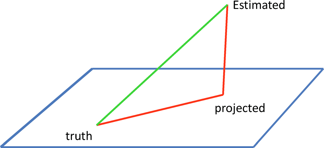
Figure 9.2: The projected matrix cannot be twice worse than the unprojected one by using the triangular inequality. In the case of a rotationally invariant norm, the projected matrix is indeed closer to the truth.

More generally, we can cast the following projection problemml:

(9.23)

where S is a set of matrices such that Σ ∈ S is a feasible solution. Let S_λ be a solution. Then, we have

Figure 9.2 gives an illustration. In other words, the projection cannot make the estimator much worse than the original one. For example, if we take the elementwise L_∞-norm ||A||=|| A||_max, then the projected estimator S_λ can not be twice as worse as the original Σ̂ _λ in terms of elementwise L_∞-norm. This minimization problem can be solved by using cvx solver in MATLAB (Grant and Boyd, 2014) for the constraint λmin(X) ≥ δ.

Another way of enforcing semi-positive definiteness is to impose a constraint on the covariance regularization problem. For example, in minimizing (9.11), we can impose the constraint λ_min(Σ) ≥ τ. Xue, Ma and Zou (2012) propose this approach for enforcing the positive definiteness in thresholding covariance estimator:

and the above eigenvalue constrained sparse covariance estimator can be solved efficiently via an alternating direction method of multiplier algorithm. A similar estimator was considered by Liu, Wang, and Zhao (2014).

9.3 Robust Covariance Inputs

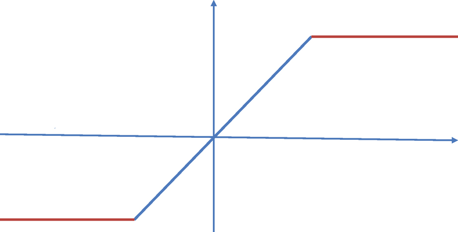
Figure 9.3: Winsorization or truncation of data.

The sub-Gaussian assumption is too strong for high-dimensional statistics. Requiring tens of thousands of variables to have all light tails is a mathematical fiction rather than reality. This is documented in Fan, Wang and Zhu (2016). Catoni (2012), Fan, Wang, Zhu (2016) and Fan, Li, and Wang (2017) tackle the problem by first considering estimation of a univariate mean /..t from a sequence of i.i.d random variables , Y_{1, ⋯}Y_n with variance σ. In this case, the sample mean Y provides an estimator but without exponential concentration. Indeed, by the Markov inequality, we have

which is tight in general and has a Cauchy tail (in terms of t). On the other hand, if we truncate the data Ỹ_i =sign(Y_i) min (|Y_i|, τ) with τ ≍ σ√n (see Figure 9.3) and compute the mean of the truncated data (usually called Win-sorized data), then we have (Fan, Wang and Zhu, 2016)

(9.24)

for a universal constant c > 0 (see also Theorem 3.2). In other words, the mean of truncated data with only a finite second moment behaves very much the same as the sample mean from the Gaussian data: both estimators have Gaussian tails (in terms of t). This sub-Gaussian concentration is fundamental in high-dimensional statistics as the sample mean is computed tens of thousands or even millions of times, and with sub-Gaussianity, the maximum error will not accumulate to be too large.

As an example, estimating the high-dimensional covariance matrix Σ — (σ_ij) involves O(p) univariate mean estimation, since the covariance can be expressed as σ_ij= E(X_iX_j) — E(X_i) E(X_j). Estimating each component by the truncated mean yields an elementwise robust covariance estimator

(9.25)

where a is the method of estimating the univariate mean. When a = T, we refer to the truncated sample mean as in (9.24) and when a = H, we refer to the adaptive Huber estimator in Theorem 3.2. For example, for the Winsorized estimator (a = T), we have

and E(X_i)^T^ = n^-1Σⁿ_k=1 sign(X_ki)min (|X_ki|τ) in (9.25). We would expect this method performs similarly to the sample covariance matrix based on the truncated data:

(9.26)

where X̃_i is the elementwise truncated data at level τ.

Assuming the fourth moment is bounded (as the covariance itself involves second moments), by using the union bound and the above concentration inequality (9.24), we can easily obtain (see the proof in Section 9.6.3)

(9.27)

and condition (9.17) is met. In other words, with robustification, when the data have merely bounded fourth moments, we can achieve the same estimation rate as the sample covariance matrix under the Gaussian data, including the regularization result in Theorem 9.1. Formally, we have

Theorem 9.4 Let u =max_i,j SD(X_iX_i) and v = max_i SD(X_i) and σ max(u, y) be bounded. Assume that log p = o(n).

1. For the elementwise truncated estimator Σ_T when σ ≍ σ√n, we have

for any a > 0 and a constant c’ > O.

2. For the elementwise adaptive Huber estimator Σ_H, when τ = √n I (alog p)σ, we have

for any a > 0 and a constant c’ > O.

Instead of using elementwise truncation, we can also apply the global truncation. Note that

which avoids the use of mean. Truncating the norm ||X_i -X_j|at τ leads to the robust U -covariance

(9.28)

which does not involve estimation of the mean due to symmetrization of X_{i -}X_j. Fan, Ke, Sun and Zhou (2018+) prove the follow result.

Theorem 9.5 Let v =½||E{X-μ){X-μ)^T} +tr(Σ)Σ+2Σ||_2. For any t>0, when τ≥ vn^½/(2t), we have

As in the proof of Theorem 9.3, the result in Theorem 9.5also implies the sharp result in elementwise L∞-norm II·||_max, namely condition (9.17).

Before the introduction of the robust U-covariance matrix estimator, Fan, Wang and Zhu (2016) and Minsker (2016) independently propose shrinkage variants of the sample covariance using fourth moments. Specifically, when EX = 0, they propose the following estimator:

(9.29)

It admits the sub-Gaussian behavior under the spectral norm, as long as the fourth moments of X are finite.

For an elliptical family of distributions, Liu, Han, Yuan, Lafferty, and Wasserman (2012) and Xue and Zou (2012) used rank correlation such as the Kendall τ correlation (9.46) or Spearman correlation and (9.49) (see Section 9.5) to obtain a robust estimation of the correlation matrix. After estimating the correlation matrix, we can use Catoni’s (2012) method to obtain robust estimation of individual variances. Such constructions also possess the uniform elementwise convergence as in Theorem 9.4.

9.4 Sparse Precision Matrix and Graphical Models

The inverse of a covariance matrix, also called a precision matrix, is prominently featured in many statistical problems. Examples include Fisher dis-criminant, Hotelling T-test, and the Markowitz optimal portfolio allocation vector. It plays an important role in Gaussian graphical models (Lauritzen, 1996, Whittaker, 2009). This section considers estimation of the sparse precision matrix and its applications to graphical models.

9.4.1 Gaussian graphical models

Let X ~ N(μ, Σ) and Ω= Σ^-1. Then, it follows that the conditional distribution of a block of elements given the other block of variables is also normally distributed. In particular, if we partition

then the conditional distribution of

(9.30)

where Σ_11.2 = Σ₁₁ — Σ₁₂Σ^-₂₂Σ₂₁ is the Schur completement of Σ₂₂.

Let Ω = Σ^-1 be the precision matrix, and , Ω₁₁, Ω_12, Ω₂₁ and Ω₂₂ be its partition in the same way as Σ. Then, it follows from the block matrix inversion formula at the end of Section 9.1, we have Ω₁₁ = Σ^-1_11.2. In particular, when X₁ = (X₁, X₂)^T and X₂ = (X3, ⋯ , X_p)^T, we can compute Σ^-1_11.2 analytically for the 2 x 2 matrix Σ_11.2. It then follows easily that

In other words, ω₁₂ = 0 if and only if X₁ and X₂ are independent given X₃, ⋯ , X_p. We summarize the result as follows.

Proposition 9.3 For a Gaussian random vector X with precision matrix Ω=(ω_ij), (ω_ij) = 0 if and only if X_i and X_i are conditionally independent, given the rest of the other random variables.

This result will be extended to the Gaussian copula in Section 9.5 and serves as the basis of the graphical model. The latter summarizes the conditional dependence network among the random variables {X_j}^P_i=1 via a graph. The vertices of the graph represent variables X₁, ⋯, X_p and the edges represent the conditional dependence. The edge between i and j exists if and only if ω_{ij #} 0. Figure 9.4 gives such an example for p = 6.

Figure 9.4: The left panel is a precision matrix and the right panel is its graphical representation. Note that only the zero pattern of the precision matrix is used in the graphical representation.

9.4.2 Penalized likelihood and M-estimation

For given data from a Gaussian distribution, its likelihood is given by (9.8). By (9.8), reparameterizing Σ by Ω = (ω_ij) and adding the penalty term to the likelihood leads to the following penalized likelihood:

(9.31)

The optimization problem (9.31) is challenging due to the singularity of the penalty function and the positive definite constraint on Ω. When the penalty is the Lasso penalty, Li and Gui (2006) used a threshold gradient descent procedure to approximately solve (9.31). Their method was motivated by the close connection between 6-boosting and Lasso. Various algorithms have been proposed to solve (9.31) with the Lasso penalty. Yuan and Lin (2007) used the maxdet algorithm but that algorithm is very slow for high-dimensional data. A more efficient clockwise descent algorithm was proposed in Baner-jee, El Ghaoui and d’Aspremont (2008) and Friedman, Hastie and Tibshirani (2008). Duchi et al. (2008) proposed a projected gradient method and Lu (2009) proposed a method by applying Nesterov’s smooth optimization technique. Scheinberg et al. (2010) developed an alternating direction method of multiplier for solving the Lasso penalized Gaussian likelihood estimator. Fan, Feng and Wu (2009) studied (9.31) with the adaptive Lasso penalty. Roth-man, Bickel, Levina and Zhu (2008) and Lam and Fan (2009) derived the asymptotic properties of the estimator. They showed that

and the consistency of sparsity selection for folded concave penalty function, where |Ω*| is the number of non-zero elements of true Ω*. Under an irrep-resentable condition, Ravikumar et al. (2011) established the selection consistency and rates of convergence of the Lasso penalized Gaussian likelihood estimator.

Zhang and Zou (2014) introduced an empirical loss minimization framework to the precision matrix estimation problemml:

(9.32)

where L is a proper loss function that satisfies two conditions:

  (i) L(Ω, Σ) is a smooth convex function of Ω;

  (ii) the unique minimizer of L(Ω, Σ*) occurs at the true Ω* = (Σ*)^-1.

Condition (i) is required for computational reasons and condition (ii) is needed to justify (9.32). In (9.31) the negative log-Gaussian likelihood is identical to the loss function Lg(Ω, Σ) = (Ω, Σ)- log det(Ω). Zhang and Zou (2014) further proposed a new loss function named D- Traceloss:

(9.33)

One can easily verify that L_D (Ω, Σ) satisfies conditions (i) and (ii). In particular, the D-Trace loss has a constant Hessian matrix of the form (Σ⊗I+I⊗Σ)/2, where ⊗ denotes the Kronecker product. For the empirical D-Trace loss LD(Ω, S) its Hessian matrix is (S ⊗ I + I ⊗ S)/2. With the D-Trace loss, (9.32) is solved very efficiently by an alternating direction method of multiplier. Selection consistency and rates of convergence of the Lasso penalized D-Trace estimator are established under an irrepresentable condition. It is interesting to see that (9.32) provides a good estimator of Σ^-1 without the normality assumption on the distribution of X. The penalized D-Trace estimator can even outperform the penalized Gaussian likelihood estimator when the data distribution is Gaussian. See Zhang and Zou (2014) for numerical examples.

9.4.3 Penalized least-squares

The aforementioned methods directly estimate the precision matrix Ω. If we relax the positive definiteness condition for Ω, a computational easy alternative is to estimate Ω via column-by-column methods. Without loss of generality, we assume μ = 0 for simplicity of presentation.

For a given j, let X_-j be the subvector of X without using X_j. Correspondingly, let Σ_j be the (p —1) x (p — 1) matrix with j^th row and j^th column deleted, and σ_j be the j^th column of Σ with the i^th element deleted. For example, when j = 1, the introduced notations are in the partition:

Set τ_j= σ_jj— σ^T_j Σ^-1_jσ_j. By (9.30), we have

(9.34)

Using the similar notations to those for Σ, we define similarly Ω_j and ω_j based on Ω By the block inversion formula at the end of Section 9.1, we have, for example,

where ^“xyz^“ is a quantity that does not matter in our calculation. Therefore, ω₁₁= τ^-1₁ and ω₁ = β₁/τ₁ with β₁ given by (9.34). Note that β₁ is the regression coefficient of X₁ given X_-1 and τ₁ is its residual variance. The sparsity of β₁ inherits from that of ω₁. Therefore, the first column can be recovered from the of X₁ the rest of the variables.

The above derivation holds for every j. It also holds for non-normal distributions, as all the properties are the results of linear algebra, rather than those of the normal distributions. We summarize the result as follows.

Proposition 9.4 Let α*_j and β^*_j; be the solution to the least-squares problemml:

Then, the true parameters Ω* are given column-by-column as follows:

Proposition 9.4 shows the relation between the matrix inversion and the least-squares regression. It allows us to estimate the precision matrix S2 column-by-column. It prompts us to estimate the j^th column via the penalized least-squares

(9.35)

This is the key idea behind Meinshausen and Biihlmann (2006) who considered the L₁-penalty. Note that each regression has different residual variance τ_j and therefore the penalty parameter should depend on j. To make this less dependence sensitive, Liu and Wang (2017) propose to use the square-root Lasso of Belloni, Chernozhukov, and Wang (2011), which minimizes

Instead of using the Lasso, one can use the Dantzig selector:

(9.36)

for a regularization parameter γ_j, where S_j and s_j is the partition of the sample covariance matrix S in a similar manner to that of Σ. This method is proposed by Yuan

Sun and Zhang (2013) propose to estimate β_j and τ_j by a sealed-Lasso: Find b̂_j and σ̂_j to minimize (to be explained below)

(9.37)

Once b̂_j and σ̂_j are obtained, we get β̂_j = (b̂_1,...,b̂_j-1, b̂_{j+1, ...,} b̂_p)^T and τ̂_j=σ̂_j. Thus, we obtain a column-by-column estimator using Proposition 9.4. They provide the spectral-norm rate of convergence of the obtained precision matrix estimator.

Note that b^TSb in (9.37) is a compact way of writing the quadratic loss in (9.35), after minimizing with respect Œ₃ (Exercise 9.9), also called profile least- squares. It also shows innately the relationship between covariance estimation and least-squares regression. Indeed,

(9.38)

We can replace Σ* by any of its robust covariance estimators in Section 9.3. This yields a robust least-squares estimator, requiring only bounded fourth moments in high-dimensional problems. In such a kind of least-squares problem, it is essential to use a semi-positive definite covariance estimate. Pro_jections in Section 9.2.3 are essential before plugging it into (9.38).

The column-by-column estimator Ω̂ is not necessarily symmetric. A simple fix is to do pro_jection:

where ||·||* can be the operator, Frobenius, or elementwise max norm. For both the Frobenius and elementwise max norms, the solution is

Another way of symmetrization is to perform a shrinkage and symmetrization simultaneously: Ω_s, (ω̂^s_ij) with

(9.39)

This was suggested by Cai, Liu and Luo (2011) for their CLIME estimator so that it has the property

(9.40)

As an illustration, we use gene expression arrays from Arabidopsis thaliana in Wille et al. (2004) and construct the genomic network that involves 39genes in two isoprenoid metabolic pathways: 16 from the mevalonate (MVA) pathway are located in the cytoplasm, 18 from the plastidial (MEP) pathway are located in the chloroplast, and 5 are located in the mitochondria. While the MVA and MEP pathways generally operate independently, crosstalks can happen too. Figure 9.5 gives the conditional dependence graph using TIGER in Lin and Wang (2017). The graph has 44 edges and suggests that the connections from genes AACT1 and HMGR2 to gene MECPS indicate a primary sources of the crosstalk between the MEP and MVA pathways.

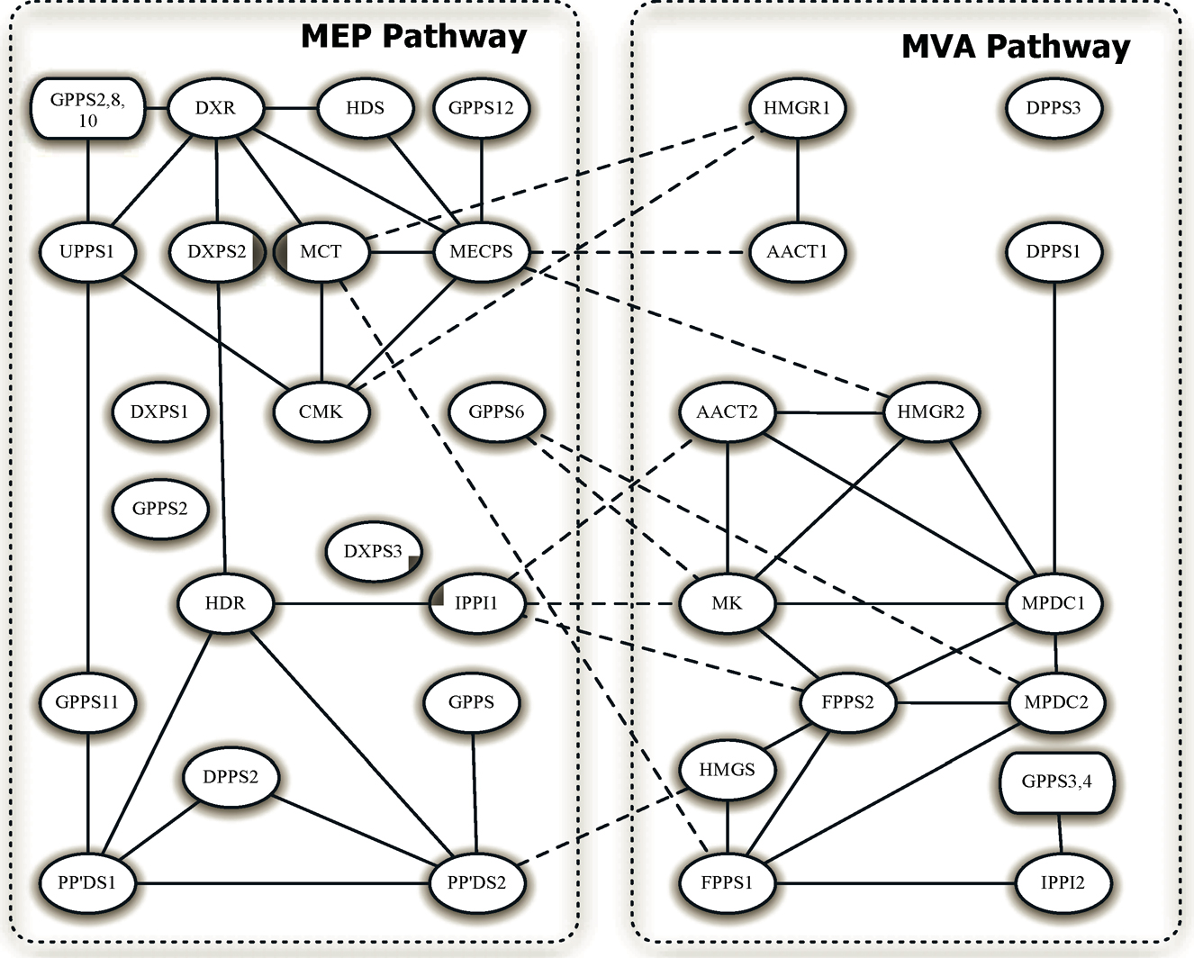
Figure 9.5: The estimated gene networks of the A ra,badopsis data. The within-pathway links are shown in solid lines and between-pathway links are presented by dashed lines. Adapted from Liu and Wang (2017).

9.4.4 CLIME and its adaptive version

For a given covariance input Σ̃, the constrained l₁-minimization for inverse matrix estimation (CLIME), introduced by Cai, Liu, and Luo (2011), solves the following problemml:

(9.41)

where Σ is a pilot estimator of Σ and ||Ω|| l1 = Σ_i,j |ω_ij| is the elementwise l₁-norm. It is used to facilitate the computation of the solution Ω̂.

Following the Dantzig-selector argument, it is interesting to see that CLIME is more closely related to the L₁-penalized D-Trace estimator in Zhang and Zou (2014). The first order optimality condition of

is ½(ΩΣ̃^- +Σ̃^-Ω) —I_p= λ_nZ, where Z_ij ∈[-1, 1]. This suggests an alternative Dantzig-selector formulation as follows:

We call the above formulation the symmetrized CLIME because it is easy to show that its solution is always symmetric, while the CLIME solution is not.

The parameter λ_n is chosen such that

(9.42)

The Dantzig-type of estimator admits a very clear interpretation: in the high-confidence set {Ω : ΣΩ ^—I_p||_max ≤ λ_n}, which has the coverage probability tending to one, let us find the sparsest solution gauged by the f_i-norm.

Let e_i be the unit vector with 1 at the j^th position. Then, the problem (9.41) can be written as

(9.43)

It can be casted as p separate optimization problems: find ω̂_i to solve

(9.44)

This problem can be solved by a linear program. Let σ̃_k be the k^th column of Σ. Write ω = ω_j (dropping the index j in ω_j) and x_i =|ω_i|where ω_i is the i^th component of ω. Then, the problem (9.44) can be expressed as

The first two constants are on the fact that x_i = |ω_i| and the last two constraints are on ||Σω_j — ej||∞ ≤ λ_n. Thus, we have 2p variables x and ω and 4p linear inequality constraints.

After obtaining the column-by column estimator, we need to symmetrize the estimator as in (9.39), resulting in Ω̂_s. Now consider a generalized sparsity measure that is similar to (9.16), namely,

Using the sample covariance as the initial estimator, Cai, Liu and Luo (2011) established the rate of convergence for the CLIME estimator. Inspecting the proof there, the results hold more generally for any pilot estimator that satisfies certain conditions, which we state below.

Theorem 9.6 If we take λ_n > ‖Ω*‖ ‖Σ-Σ‖max, then uniformly over true precision matrix Ω* ∈ C_q^* (m_p),

In particular, if the pilot estimator Σ̅̃ satisfies

(9.45)

with probability at least 1 — ε_n,p, by taking λ_n = C₀D_n√(log p)/n, we have

The results in Theorem 9.6 indicate that any pilot estimator that satisfies (9.45) can be used for CLIME regularization. In particular, the robust covariance inputs in Section 9.3 are applicable.

The CLIME above uses a constant regularization parameter λ_n, which is not ideal. Cai, Liu and Zhou (2016) introduce an adaptive version, called ACLIME. It is based on the observation that the asymptotic variance of (SΩ — I_p)_ij in (9.41) is heteroscedastic and depends on σ_iiω_jj for the sample covariance matrix S. Therefore, the regularization parameter should be of form

which depends on unknown quantities σ_ii and ω_ii. These unknown quantities need to be estimated first.

Fan, Xue and Zou (2014) show that the CLIME estimator can be used as a good initial estimator for computing the SCAD penalized Gaussian likelihood estimator such that the resulting estimator enjoys the strong oracle property. Recall that the SCAD penalized Gaussian likelihood estimator of Ω is defined as

Let A denote the support of the true Ω*. The oracle estimator of Ω* is defined as

Let Ω⁽⁰⁾ be the CLIME estimator and compute the following weighted ℓ₁ penalized Gaussian likelihood estimator for k =1, 2

Fan, Xue and Zou (2014) show that with an overwhelming probability Ω⁽²⁾ equals the oracle estimator. Simulation examples in Fan, Xue and Zou (2014) also show that Ω⁽²⁾ performs better than the Lasso penalized Gaussian likelihood estimator and CLIME.

Avella-Medina, Battey, Fan and Li (2018) generalize the procedure to a general pilot estimator of covariance, which includes robust covariance inputs in Section 9.3. It adds a projection step to the original ACLIME. The method consists of the following 4 steps. The first step is to make sure that the covariance input Σ⁺ is positive definite. The second step is a preliminarily regularized estimator to get a consistent estimator for ω_jj. It can be a non-adaptive version too. The output ω_jj⁽¹⁾ is to make the mathematical argument valid. The third step is the implementation of the adaptive CLIME that takes into account of the aforementioned heteroscedacity. The last step is merely a symmetrization.

1. Given a covariance input Σ̃, let

for an small ε > 0. This can be easily implemented in MATLAB using the cvx solver, as mentioned in Section 9.2.3. We then estimate σ_ii by σ_ii⁺, the i^th diagonal element of the projected matrix Σ⁺.

2. Get an estimate of {w_jj} by using CLIME with an adaptive regularization parameter via solving

This is still a linear program. Output

3. Run the CLIME with adaptive tuning parameter

4. The final estimator is constructed as the symmetrization of the last estimator:

Avella-Medina et al. (2018) derive the asymptotic property for the ACLIME estimator with a general covariance input that satisfies (9.17). The results and the proofs are similar to those in Theorem 9.6.

Avella-Medina et al. (2018) conduct extensive simulation studies and show the big benefit of using robust covariance estimators as a pilot estimator, for both estimating the covariance matrix and the precision matrix. In particular, they used the elementwise adaptive Huber estimator in their simulation studies.

To assess whether their proposed robust estimator can improve inference on gene regulatory networks, they used a microarray dataset in the study by Huang et al. (2011) on the inflammation process of cardiovascular disease. Huang et al. (2011) found that the Toll-like receptor signaling (TLR) pathway plays a key role in the inflammation process. Their study involves n = 48 patients and data is available on the Gene Expression Omnibus via the accession name “GSE20129” . Avella-Medina et al. (2018) considered 95 genes from the TLR pathway and another 62 genes from the PPAR signaling pathway which is known to be unrelated to cardiovascular disease. We would expect that a good method discovers more connections for genes within each of their pathways but not across them. In this study, n = 48 and p = 95 + 62. To see whether a robust procedure gives some extra merits, they used both the adaptive Huber estimator and the sample covariance matrix as pilot estimators. We will call them robust ACLIME or “RACLIME” and ACLIME, respectively.

They first chose the tuning parameters that deliver the top 100 connections for each method. The selection results are presented in the left panel in Table 9.1 and also displayed graphically in Figure 9.6. The robust ACLIME identifies a greater number of connections within pathways and fewer connections across pathways.

They additionally took the same tuning parameter in the ACLIME optimization problem for each procedure. The results are summarized in the right panel of Table 9.1. The robust procedure detects fewer connections, but yields higher percentage (64.2% by robust ACLIME) of within-pathway connections (in comparison with 55% by ACLIME).

Table 9.1: Summary of regulatory network graphs: Number of connections detected by using robust ACLIME and regular ACLIME, with two methods of choosing regularization parameters. Adapted from Avella-Medina et al. (2018).

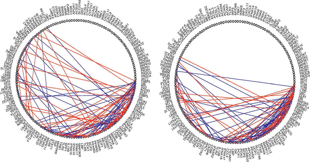
Figure 9.6: Connections estimated by ACLIME using the sample covariance pilot estimator (left) and the adaptive Huber type pilot estimator (right). Blue lines are within pathway connections and red lines are between pathway connections. Taken from Avella-Medina et al. (2018).

9.5 Latent Gaussian Graphical Models

Graphical models are useful representations of the dependence structure among multiple random variables. Yet, the normality assumption in the last two sections is restrictive. This assumption has been relaxed to the Gaussian copula model by Xue and Zou (2012) and Liu, Han, Yuan, Lafferty, and Wasserman (2012). It has been further extended by Fan, Liu, Ning, and Zou (2017) to binary data and the mix of continuous and binary types of data. In particular, the method allows one to infer about the latent graphical model based only on binary data. This section follows the development in Fan et al. (2017).

Definition 9.4 A random vector X (X₁, …, X_p)^Tis said to follow a Gaussian copula distribution, if there exists strictly increasing transformations g=(g_j)_j^p=1 such that g(X) (g₁(X₁),…,gp(X_p))^T~ N(0, Σ) with σ_jj=1 for any 1 ≤ j ≤ p. Write X ~ NPN(0, Σ, g), also called a nonpara-normal model.

In the above definition, we assume without loss of generality that Σ is a correlation matrix. This is due to the identifiability: the scale of functions Σ can also be taken such that Σ is a correlation matrix. Let F_j(·) be the cumulative distribution function of a continuous random variable X_j. Then, F_j(X_j) follows the standard uniform distribution and Φ⁻¹(F_j(X_j)) ~ N(0, 1), where Φ(·) is the cdf of the standard normal distribution. Therefore,

and can easily be estimated by substitution of its empirical distribution F̂_n,j(·) or its smoothed version. Therefore, Ω can be estimated as in the previous two sections using the transformed data {ĝ(X_i)}_iⁿ=1.

It follows from Proposition 9.3 that g_i(X_i) and g_i(X_i) given the rest of the transformed variables are independent if and only if W_ij= 0. Since the functions in g are strictly increasing, this is equivalent to the statement that X_i and X_j are independent given the rest of the untransformed data.

Proposition 9.5 If X ~ NPN(0, Σ, g), then X_i and X_i are independent given the rest of the variables in X if and only if W_ij =0. In addition, g_j(x) = Φ⁻¹(Fi(x)).

There are several ways to model binary data. One way is through the Ising model (Ising,1925). Ravikumar, Wainwright and Lafferty (2010) proposed the neighborhood Lasso logistic regression estimator for estimating the sparse Ising model. The Lasso and SCAD penalized composite likelihood estimators were considered in Höfling and Tibshirani (2009) and Xue, Zou and Cai (2012), respectively. Another way is to dichotomize the continuous variables. This leads us to the following definition for the data generation process for the mix of binary and continuous type of data. In particular, it includes all binary data as a specific example.

Definition 9.5 Let X= (X₁^T, X₂^T)^T, where X₁ represents d₁-dimensional binary variables and X₂ represents d₂-dimensional continuous variables. The random vector X is said to follow a latent Gaussian copula model, if there exists a d₁-dimensional random vector Z₁ (Z₁, … , Z_p1)^T such that Z= (Z₁, X₂) ~ NPN(0, Σ, g) and

where II[(·) is the indicator function and C = (C₁, , C_p1) is a vector of constants. Denote by X ~ LNPN(0, Σ, g, C), where Σ is the latent correlation matrix.

Based on the observed data of mixed types, we are interested in estimating Ω and hence the conditional dependence graph of latent variables Z. To obtain this, we need a covariance input that satisfies (9.17) so that the methods introduced in the previous two sections can be used. For continuous variables, its covariance can be estimated by using the estimated transformations (Liu et al., 2012; Xue and Zou, 2012). For binary data and binary-continuous data, how to estimate their covariance matrices is unclear.

Fan, Liu, Ning and Zou (2017) provide a unified method to estimate the covariance matrix for mixed data, including continuous data, using the Kendall τ correlation

(9.46)

It estimates the population quantity

(9.47)

using sgn(ab) = sgn(a)sgn(b).

For binary data a and b, using sgn(a — b) = a — b, it follows from (9.47) that

Let Δ_j = g_j (C_j) and Φ₂ (x₁, x₂, ρ) be the cumulative distribution function of the bivariate normal distribution with mean 0 and correlation ρ. Then, since g_j (·) is strictly increasing and g_j (Z_ij) ~ N(0, 1), we have

(9.48)

Note that P(X_j= 1) =ΦΔ_j. This leads to a natural estimator

Note that Φ₂ (x₁, x₂, ρ) is a strictly increasing function of ρ. Hence, we can estimate σ_ij via the inversion of (9.48).

For continuous data, note that

and (U_j, U_k) follow the bivariate normal distribution with mean 0 and correlation ρ. Thus, by (9.47), we have

(9.49)

or

The latter was shown in Kendall (1948) that spells out the relationship between Kendall’s τ-correlation and Pearson’s correlation. This forms the basis of the rank based covariance matrix estimation in Liu et al. (2012) and Xue and Zou (2012). Note that the relation (9.49) holds for elliptical distributions or more generally the transformations of elliptical distributions (Liu, Han, and Zhang, 2012; Han and Liu, 2017). We leave this as an exercise.

Now, for the binary and continuous blocks of the covariance matrix, similar calculation shows (Exercise 9.13) that

(9.50)

where we assume that X_j is binary and X_k is continuous.

Proposition 9.6 Suppose the mixed data {X_i}_i=1ⁿ are drawn from X~ LNPN(0, Σ, g, C). Then, the relation between Kendall’s τ correlation and Pearson’s correlation are given by τ_ij= G(σ_ij), where the function G(·) is given respectively in (9.48), (9.49) and (9.50), for binary, continuous and binary-continuous blocks.

Now a natural initial covariance estimator is Σ in which σ̃_jk= G⁻¹(τ̂_jk) for j ≠ k and σ̃_jj= 1. It is easy to show that G⁻¹(x) is a Lipschitz function of x, for |x| ≤ c, for any constant c < 1. Therefore, the concentration inequality of σ̃_jk follows from that of τ̂_ij , which is established in Fan, Liu, Ning and Zou (2017). The basic idea in establishing the concentration inequality is that Δ_j and τ_jk can be uniformly estimated by using the Hoeffding inequality for p̂_j and the U-statistics τ̂_ij. As a result, they showed that the pilot estimator satisfies condition (9.17):

With this pilot covariance estimator, we can now estimate the precision matrix using the methods in the previous two sections and construct the corresponding conditional graph.

9.6 Technical Proofs

9.6.1 Proof of Theorem 9.1

By (9.14), we need to bound individual L₁-error. Consider the event E₁= {|(σ̂_ij — σ̂_ij| ≤ λ_ij/2,∀_{i, j}}. For this event, we have

by using the property of the generalized thresholding function (see Definition 9.3b)). Thus, by considering the cases Iσ̂_ijI ≥ λ_ij and Iσ̂_ijI < λ_ij separately and using property a) of the generalized thresholding function for the second case, we have that for the event E₁,

(9.51)

Hence, we have

which is bounded, for the event E₂ = Iσ̂̂_iiσ̂̂_jjI ≤ 2σ̂̂_iiσ̂̂_jj, ∀_i, j}, further by

by using the definition of (9.13). Hence, for the parameter space C_q(m_p), we have by using (9.14) that

for a constant C₁ (2.5 + a)(2Cλ)^1−q.

It remains to lower bound the probability of the event ε_n ={E₁ ⋂ E₂}. Notice that

(9.52)

Since the last three terms tend to zero and σ_ii ≥ γ, it therefore follows from (9.17) that, for large n

Consequently,

where the last one follows from (9.17) when λ is sufficiently large. Hence, we have

This completes the proof of the first result.

The proof of the second result follows a similar calculation. Using the same calculation as in (9.51), replacing q there by q/2, we have for the event E₁

Hence, for the event E₂, using σ_ii, ≤ C₂, we have

where C₃ = (2.5 + a)²(2λ)^2−qC₂. This completes the proof.

9.6.2 Proof of Theorem 9.3

We plan to use Theorem 9.2 to prove this theorem. Consider a 2 × 2 submatrix S_ij of S that involves s_ij. Then, the corresponding κ_ij is bounded by κ by definition. Similarly, the corresponding

which is bounded by assumption. Hence, the constant c_ij is lower bounded by some c > 0 and the constant _Cij is upper bounded by a constant C. Thus, for sufficiently large t that is bounded by √n/2,

Now applying Theorem 9.2 to this 2 × 2 submatrix S_ij, we obtain

Now, take t = √a log p = 0(√n), we obtain

By the union bound, we have

which tends to zero by taking a is a sufficiently large constant. This completes the proof.

9.6.3 Proof of Theorem 9.4

By using (9.24), for the truncated estimator, with t = √(a/c) logp, we have

and similarly

Therefore, by the union bound, we have P(E₁^c) < 2p^2−a, where

and P(E₂^c) ≤ 2p^1−a, where

Using the decomposition (9.52) and log p = o(n), when n is sufficiently large, for the event E₂, we have

Therefore, for the event E₁ ⋂ E₂, we have

The result now follows from the fact that

by taking c′ = c/(1 + 3 max_i E |X_i|)².

The same proof applies to the elementwise adaptive Huber estimator by using the concentration inequality in Theorem 3.2 d). For example, with t = √alog p, we have τ = √n/(a log p)σ and

The rest follows virtually the same line of the proof.

9.6.4 Proof of Theorem 9.6

Let Ω* and Σ^* be the true precision and covariance matrices, respectively.

(i) Let us first establish the result under ‖·‖_max norm. Using ‖AB‖_max ≤ ‖A‖_max ‖B‖₁, we have

This shows that Ω* is in the feasible set of (9.41) or equivalently (9.43). Let ω_j^* and ω̂_j^* be respectively the j^th column of Ω^* and Ω̂. Since ω_j^* is a feasible solution to the problem (9.43), we have ‖ω̂_j^*‖₁ ≤ ‖ω̂_j^*‖₁ by the equivalent optimization problem (9.44). Hence, ‖Ω̂‖₁ ≤ ‖Ω_j^*‖₁ By (9.40), we have

(9.53)

The triangular inequality entails that

where we used the fact that Ω̂_s satisfies the constraint in (9.41). The inequality (9.53) implies that ‖Ω_s — Ω*‖₁ ≤ 2‖Ω^*‖₁ and it follows from the last result that

Therefore, we conclude that

where the last inequality uses again from ‖AB‖_max≤‖A‖_max‖B‖_1.

(ii) We next consider the loss under the operator norm. Recall that ‖Ω̂_s− Ω*‖₂ ≤‖Ω̂_s — Ω^*‖₁. Thus, it suffices to bound the matrix L₁-norm. Let

where a_n = ‖Ω̂_s - Ω^*‖_max. Let ω̂̂_j¹, ω̂_j² and ω̂̂_j^s be the j^th column of Ω̂₁, Ω̂₂, Ω̂_s, respectively. Then, by (9.40), we have

On the other hand,

The combination of the last two displays leads to

In other words, ‖Ω̂₂ ‖≤ Ω̂₁ — Ω*‖₁.Hence,

It remains to bound the estimation error ‖Ω̂₂ −Ω*‖₁. This is indeed a hard-thresholding estimator Ω₁ for the sparse matrix Ω*. The results then follow from the proof of Theorem 9.1, which requires only sparsity and uniform consistency of the pilot estimator. More specifically, note that for the hard-thresholding function, we have a = 2. Adopting (9.51) to the current setting, we have λ_ij = 2a_n there. Set d_ij= |ω̂ ^s_ijII ω̂ ^s_ij| ≥ 2a_n)-ω_ij*|. It follows from property b) of Definition 9.3 with a = 2 that

Now, separating the bounds for two cases with II{ |ω_ij*| ≥ a_n} and II{ |ω_ij*| < a_n}, using the property a) of Definition 9.3 for the second case for the hard-thresholding function, we have

Hence,

using Ω* ∈ C_q^* (mp) namely, ‖Ω₁ − Ω*‖ ≤ 6a_n^1-q m_p. Therefore,

(iii) The result for the Frobenius norm follows immediately from that

and the results in (i) and (ii).

For the event (‖Σ — Σ‖ _max > C₀ √(log p) /n) , the second part of the result follows directly from the choice of λ_n and the fact ‖Ω‖₁ ≤ D_n. This completes the proof.

9.7 Bibliographical Notes

Wu and Pourahmadi (2003) gave a nonparametric estimation for large covariance matrices of longitudinal data. Estimation of a high-dimensional covariance matrix was independently studied by Bickel and Levina (2008a,b) for banded and sparse convariance and Fan, Fan, and Lv (2008) for low-rank plus diagonal matrix. Levina, Rothman and Zhu (2008) and Lam and Fan (2009) investigated various maximum likelihood estimators with different sparse structures. Xue, Ma and Zou (2012) derived an efficient convex program for estimating a sparse covariance matrix under the positive definite constraint. Xue and Zou (2014) showed an adaptive minimax optimal estimator of sparse correlation matrices of a semiparametric Gaussian copula model. The optimality of large covariance estimation was investigated by Cai, Zhang and Zhou (2010), Cai and Liu (2011), Cai and Zhou (2011, 2012a, b), Rigollet and Tsybakov (2012), Cai, Ren, and Zhou (2013), among others. Gao, Ma, Ren, and Zhou (2015) investigated optimal rates in sparse canonical correlation analysis. Cai and Yuan (2012) studied an adaptive covariance matrix estimation through block thresholding. Bien, Bunea, and Xiao (2016) proposed convex banding, Yu and Bien (2017) considered a varying banded matrix estimation problem, and Bien (2018) introduced a generalized notation of sparsity and proposed graph-guided banding of the covariance matrix. Xue and Zou (2014) proposed a ranked-based banding estimator for estimating the bandable correlation matrices. Li and Zou (2016) proposed a Stein’s Unbiased Risk Estimation (SURE) criterion for selecting the banding parameter in the banded covariance estimator. Additional references can be found in the book by Pourahmadi (2013).

There is a large literature on estimation of the precision matrix and its applications to graphical models. An early study on the high-dimensional graphical model is Meinshausen and Bühlmann (2006). Penalized likelihood is a popular approach to this problem. See for example Banerjee, El Ghaoui and d’Aspremont (2008), Yuan and Lin (2007), Friedman, Hastie and Tibshirani (2008), Levina, Rothman and Zhu (2008) and Lam and Fan (2009), Fan, Feng and Wu (2009), Yuan (2010), Shen, Pan and Zhu (2012). Ravikumar, Wainwright, Raskutti, and Yu (2011) proposed estimating the precision matrix by the penalized log-determinant divergence. Zhang and Zou (2014) proposed the penalized D-trace estimator for sparse precision matrix estimation. Cai, Liu and Luo (2011) and Cai, Liu and Zhou (2016) proposed a constrained ℓ₁ minimization approach and its adaptive version to sparse precision matrix estimation. Liu and Wang (2017) proposed a tuning-insensitive approach. Ren, Sun, Zhang and Zhou (2015) established the asymptotic normality for entries of the precision matrix and obtained optimal rates of convergence for general sparsity. The results were further extended to the situation where heterogeneity should be adjusted first before building a graphical model in Chen, Ren, Zhao, and Zhou (2016).

The literature has been further expanded into robust estimation based on regularized rank-based approaches (Liu, Han, Yuan, Lafferty, and Wasserman, 2012; Xue and Zou, 2012). The related work includes, for instance, Mitra and Zhang (2014), Wegkamp and Zhao (2016), Han and Liu (2017), Fan, Liu, and Wang (2018). It requires elliptical distributions on the data generating process. Such an assumption can be removed by the truncation and adaptive Huber estimator; see Avella-Medina, Battey, Fan, and Li (2018).

9.8 Exercises

9.1 (a) Suppose that A and B are two invertible and compatible matrices. Show that for any matrix norm

Hint: Use A⁻¹ — B⁻¹ = A⁻¹(B — A)B⁻¹.

(b) Suppose that the operator norms ‖Σ‖ and ‖Σ⁻¹‖ are bounded. If there is an estimate Σ such that ‖Σ − Σ‖ = O_P(a_n) for a sequence a_n →* 0, show that Σ̂ ⁻¹ is invertible with probability tending to 1 and that

9.2 Suppose Σ is a p × p covariance matrix of a random vector X (X₁, X₂, … X_p)^T

(a) Prove the second part of Theorem 9.1: If max_1≤i≤p σ_ii ≤ C₂, uniformly over C_q(m_p)

You may use the notation and results proved in the first part of Theorem 9.1.

(b) Assume that E(X_i) = 0 for all i, and σ = max_i,j SD(X_iX_j) is bounded. Consider the elementwise adaptive Huber estimator Σ_H = (σ̂_ij^τ) where σ̂_ij^τ is the adaptive Huber estimator of the mean E(X_iX_j) = σ_ij based on the data {X_kiX_kj}_k=1ⁿ with parameter τ. Show that when τ = √n/(a log p)σ, we have

for any constant a > 0. Hint: Use Theorem 3.2(d) of the book.

9.3 Deduce Theorem 9.3 from Theorem 9.2.

Hint: Consider a 2 × 2 submatrix that involves s_ij and apply Theorem 9.2.

The solution is furnished in Section 9.6, but it is a good practice to carry out the proof on your own.

9.4 Complete the proof of the second part of Theorem 9.4.

9.5 Use Theorem 9.5 to show that

9.6 Suppose that the covariance input Σ̂ _λ satisfies P{‖Σ_λ — Σ‖ _max ≥ a_n} ≤ ε_n. Show that the projected estimator S_λ that minimizes (9.23) with ‖·‖_max norm satisfies

9.7 Let X ~ N(µ, Σ) and Ω = Σ^-1 be the precision matrix. Let ω_ij be the (i j)^th element of Ω. Show that X_i and X_j are independent given the rest of the variables in X if and only if ω_ij =0.

9.8 This exercise intends to give a least-squares interpretation of (9.30).

(a) Without the normality assumption, find the best linear prediction of X₁ by a+ BX₂. Namely, find a and B to minimize E ‖ X₁— a — BX₂ ‖². Let a* and B* be the solution. Show that

where cov(X₂, X₁) = E(X₂—EX₂)(X₁—EX₁)^T and Var(X₂) = E(X₂-EX₂)(X₂ —EX₂)^T.

(b) Let U = X₁ — a* — B* X₂ be the residuals. Show that E U = 0 and the covariance between X₂ and U is zero:

(c) Show that

9.9 Let S be the sample covariance matrix of data {X_i}_iⁿ= 1. Show that

subject to the constraint that β_j = —1.

9.10 Prove Proposition 9.4.

9.11 Consider the optimization problem:

For both the Frobenius norm ‖· ‖_* =‖· ‖_F and elementwise max norm ‖· ‖_* =‖· ‖_max, show that the solution is

9.12 Let F(·) be the cumulative distribution function of a continuous random variable X.

(a) If _g(X)~N(0, 1), show that g(·) =Φ^-1(F(·)), where Φ(·) is the cumulative distribution function of the standard normal distribution.

(b) Let F̂_n(x) = n⁻1Σ_i=1ⁿII(X_i≤x) be the empirical distribution based on a random sample {X_i}_i=1ⁿ and ĝ_n(x) = Φ⁻¹(F̂_n(x)). Show that

where ø(·) = Φ′(·) is the density of the standard normal distribution.

9.13 We use the notation introduced in Section 9.5.

  (a) Show that the function Φ₂ (x₁, x₁,ρ) is strictly increasin_g in ρ.

  (b) Prove (9.49).

  (c) Prove (9.50).

9.14 This is a simplified version of the next exercise.

  (a) Prove the result in Exercise 9.15(b) for continuous data, rather than the mixed data.

  (b) Prove the result in Exercise 9.15(b) for binary data, rather than the mixed data.

9.15 Let the function G be defined in Proposition 9.6.

  (a) Show that G⁻¹(x) satisfies

for a sufficiently lar_ge constant D, where 0 < c < 1.

  (b) Let σ̃_jk = G⁻¹(τ̂_jk). Prove that

9.16 Download the mice protein expression data from UCI Machine Learning Repository:

https://archive.ics.uci.edu/ml/datasets/Mice+protein+ Expression.

There are in total 1080 measurements. Use attributes 2-78 (the expression levels of 77 proteins), as the input variables for large covariance estimation. We clean the missing values by dropping 6 columns “BAD_N”, “BCL2_N”, “pCFOS_N”, “H3AcK18_N”, “EGR1_N”, “H3MeK4_N” and then removing all rows with at least 1 missing value. For your convenience, you can also download directly the clean input data from the book website. You should have an input data of size 1047 × 71.

(a) Compute the correlation-thresholded covariance estimate with λ = 4. Report the entries of zeros and the minimum and maximum eigenvalues of the resulting estimate. Compare them with those from the input covariance matrix.

(Hint: the entry-dependence thresholds for the covariance matrix are

(b) Estimate the precision matrix by CLIME. (Hint: you can use the package “flare”.)

(c) Construct the protein network by using the estimated sparsity pattern of the precision matrix. (Hint: you can use the package “graph” or “ggraph”)

(d) Use the winsorized data to repeat part (a), where the winsorized parameter is taken to be 2.5 standard deviation.