3

The Size and Power of the Variance Ratio Test in Finite Samples: A Monte Carlo Investigation

3.1 Introduction

WHETHER OR NOT an economic time series follows a random walk has long been a question of great interest to economists. Although its origins lie in the modelling of games of chance, the random walk hypothesis is also an implication of many diverse models of rational economic behavior.¹ Several recent studies have tested the random walk theory of exploiting the fact that the variance of random walk increments is linear in the sampling interval.² Therefore the variance of, for example, quarterly increments must be three times as large as the variance of monthly differences. Comparing the (per unit time) variance estimates from quarterly to monthly data will then yield an indication of the random walk's plausibility. Such a comparison may be formed quantitatively along the lines of the Hausman (1978) specification test and is developed in Lo and MacKinlay (1988b). Due to intractable nonlinearities, the sampling theory of Lo and MacKinlay is based on standard asymptotic approximations.

In this chapter, we investigate the quality of those approximations under the two most commonly advanced null hypotheses: the random walk with independently and identically distributed Gaussian increments, and with uncorrelated but heteroskedastic increments. Under both null hypotheses, the variance ratio test is shown to yield reliable inferences even for moderate sample sizes. Indeed, under a specific heteroskedastic null the variance ratio test is somewhat more reliable than both the Dickey-Fuller t and Box-Pierce portmanteau tests.

We also compare the power of these tests against three empirically interesting alternative hypotheses: a stationary AR(1) which has been advanced as a model of stock market fads, the sum of this AR(1) and a pure random walk, and an ARIMA(1, 1, 0) which is more consistent with stock market data. Although the Dickey-Fuller t-test is more powerful than the Box-Pierce Q-test against the first alternative and vice versa against the second, the variance ratio test is comparable to the most powerful of the two tests against the first alternative, and more powerful against the second two alternatives when the variance ratio's sampling intervals are chosen appropriately.

Since the random walk is closely related to what has come to be known as a ‘unit root’ process, a few comments concerning the variance ratio test's place in the unit root literature are appropriate. It is obvious that the random walk possesses a unit root. In addition, random walk increments are required to be uncorrelated. Although earlier studies of unit root tests (e.g., Dickey and Fuller, 1979,1981) also assumed uncorrelated increments, Phillips (1986, 1987), Phillips and Perron (1988), and Perron (1986) show that much of those results obtain asymptotically even when increments are weakly dependent.³ Therefore, the random walk model is a proper subset of the unit root null hypothesis. This implies that the power of a consistent unit root test against the random walk hypothesis will converge to the size of the test asymptotically.

The focus of random walk tests also differs from that of the unit root tests. This is best illustrated in the context of Beveridge and Nelson's (1981) decomposition of a unit root process into the sum of a random walk and a stationary process.⁴ Recent applications of unit root tests propose the null hypothesis that the random walk component does not exist, whereas tests of the random walk have as their null hypothesis that the stationary component does not exist.⁵

Since there are some important departures from the random walk that unit root tests cannot detect, the variance ratio test is preferred when the attribute of interest is the uncorrelatedness of increments. Moreover, in contrast to the dependence of the unit root test statistics' distributions on nuisance parameters, the variance ratio's limiting distribution is Gaussian and independent of any nuisance parameters.⁶ Although we report simulation results for the Dickey-Fuller t and the Box-Pierce Q-tests for comparison with the performance of the variance ratio test, we emphasize that these three tests are not direct competitors since they have been designed with different null hypotheses in mind.

The chapter is organized as follows. In Section 3.2 we define the variance ratio statistic, summarize its asymptotic sampling theory, and define the Dickey-Fuller and Box-Pierce tests. Section 3.3 presents Monte Carlo results for the three tests under two null hypotheses, and Section 3.4 contains the power results for the three alternative hypotheses. We summarize and conclude in Section 3.5.

3.2 The Variance Ratio Test

Since the asymptotic sampling theory for the variance ratio statistic is fully developed in Lo and MacKinlay (1988b), we present only a brief summary here. Let X_t denote a stochastic process satisfying the following recursive relation:

or

where the drift µ is an arbitrary parameter. The essence of the random walk hypothesis is the restriction that the disturbances are serially uncorrelated or that innovations are unforecastable from past innovations. We develop our test under two null hypotheses which capture this aspect of the random walk: independently and identically distributed Gaussian increments, and the more general case of uncorrelated but weakly dependent and possibly heteroskedastic increments.

3.2.1 The IID Gaussian Null Hypothesis

Let the null hypothesis H₁ denote the case where the 's are IID normal random variables with variance σ². Hence

In addition to homoskedasticity, we have made the assumption of independent Gaussian increments as in Dickey and Fuller (1979, 1981) and Evans and Savin (1981a, 1981b, 1984).⁷ Suppose we obtain nq + 1 observations X₀, X₁…, X_nq of X_t, where both n and q are arbitrary integers greater than one. Consider the following estimators for the unknown parameters µ and σ²:

The estimator is simply the sample variance of the first-difference of X_t; it corresponds to the maximum likelihood estimator of the parameter σ² and therefore possesses the usual consistency, asymptotic normality and efficiency properties.

Consider the variance of qth differences of X_t which, under H₁, is q times the variance of first-differences. By dividing by q, we obtain the estimator (q) which also converges to σ² under H₁, where

We have written (q) as a function of q (which we term the aggregation value) to emphasize the fact that a distinct alternative estimator of σ² may be formed for each q.⁸ Under the null hypothesis of a Gaussian random walk, the two estimators and (q) should be ‘close’; therefore a test of the random walk may be constructed by computing the difference M_d(q) = and checking its proximity to zero. Alternatively, a test may also be based upon the dimensionless centered variance ratio which converges in probability to zero as well.⁹ It is shown in Lo and MacKinlay (1988b) that M_d(q) and M_r(q) possess the following limiting distributions under the null hypothesis H₁:

An additional adjustment that may improve the finite-sample behavior of the test statistics is to use unbiased estimators and in computing M_d(q) and M_r(q), where

with

We denote the resulting adjusted specification test statistics and . Of course, although the variance estimators and are unbiased, only is unbiased; is not.

3.2.2 The Heteroskedastic Null Hypothesis

Since there is already a growing consensus that many economic time series possess time-varying volatilities, we derive a version of our specification test of the random walk model that is robust to heteroskedasticity. As long as the increments are uncorrelated, the variance ratio must still converge to one in probability even with heteroskedastic disturbances. Heuristically, this is simply because the variance of the sum of uncorrelated increments must still equal the sum of the variances. Of course, the asymptotic variance of the variance ratios will depend on the type and degree of heteroskedasticity present. By controlling the degree of heterogeneity and dependence of the process, it is possible to obtain consistent estimators of this asymptotic variance. To relax the IID Gaussian restriction of the 's, we follow White's (1980) and White and Domowitz's (1984) use of mixing and moment conditions to derive heteroskedasticity-consistent estimators of our variance ratio's asymptotic variance. We require the following assumptions on {}, which form our second null hypothesis:

H₂:

(Al) For all t, E[] = 0, E[ _t–τ] = 0 for any τ ≠ 0.

(A2) {} is ψ-mixing with coefficients ψ(m) of size r/(2r – 1) or is α-mixing with coefficients α(m) of size r/(r – 1), r > 1, such that for all t and for any τ ≥ 0, there exists some δ > 0 for which

(A3)

(A4) For all for any nonzero j, k where j ≠ k.

 

Assumption (Al) is the essential property of the random walk that we wish to test. Assumptions (A2) and (A3) are restrictions on the degree of dependence and heterogeneity which are allowed and yet still permit some form of law of large numbers and central limit theorem to obtain. This allows for a variety of forms of heteroskedasticity including deterministic changes in the variance (due, for example, to seasonal components) as well as Engle's (1982) ARCH processes (in which the conditional variance depends upon past information).¹⁰ Assumption (A4) implies that the sample autocorrelations of are asymptotically uncorrelated.¹¹ Under the null hypothesis H₂, we may obtain heteroskedasticity-consistent estimators of the asymptotic variance δ(j) of the autocorrelations (j) of X_t. Using the fact that the variance ratio may be written as an approximate linear combination of autocorrelations (see (3.2.12) below) yields the following limiting distribution for :¹²

where

Tests of H₁ and H₂ may then be based on the normalized variance ratios z₁(q) and z₂(q), respectively, where

3.2.3 Variance Ratios and Autocorrelations

To develop some intuition for the variance ratio, observe that for an aggregation value q of 2, the M_r(q) statistic may be re-expressed as

Hence for q = 2 the M_r(q) statistic is approximately the first-order autocorrelation coefficient estimator (1) of the differences of X. More generally, we have the following relation for q ≥ 2:

where denotes terms which are of order smaller than in probability. Equation (3.2.12) provides a simple interpretation for the variance ratio computed with an aggregation value q: it is (approximately) a linear combination of the first q – 1 autocorrelation coefficient estimators of the first differences with arithmetically declining weights. Note the similarity between this and the Box-Pierce (1970) Q statistic of order q – 1,

which is asymptotically distributed as χ² with q – 1 degrees of freedom.¹³ Using (3.2.9c) we can also construct a heteroskedasticity-robust Box-Pierce statistic in the obvious way, which we denote by Q₂(q – 1). Since the Box- Pierce Q-statistics give equal weighting to the autocorrelations and are computed by squaring the autocorrelations, their properties will differ from those of the variance ratio test statistics.

For comparison, we also employ the Dickey-Fuller t-test. This involves computing the usual t-statistic under the hypothesis β = 1 in the regression

and using the exact finite-sample distribution tabulated by Fuller (1976), Dickey and Fuller (1979, 1981), and Nankervis and Savin (1985).^{14, 15}

3.3 Properties of the Test Statistic under the Null Hypotheses

To gauge the quality of the asymptotic approximations in Section 3.2, we perform simulation experiments for the statistic under both the Gaussian IID null hypothesis and a simple heteroskedastic null. More extensive simulation experiments indicate that tests based upon the unadjusted statistic M_r(q) generally yield less reliable inferences, hence, in the interest of brevity, we only report the results for . For comparison, we also report the results of Monte Carlo experiments performed for the Box-Pierce Q-statistics and the Dickey-Fuller t-statistic. All simulations are based on 20,000 replications.¹⁶

3.3.1 The Gaussian IID Null Hypothesis

Tables 3.1a and 3.1b report the results of simulation experiments conducted under the independent and identically distributed Gaussian random walk null H₁. The results show that the empirical sizes of two-sided 5 percent variance ratio tests based on either the z₁(q)- or z₂(q)-statistics are close to their nominal values for sample sizes greater than 32. Not surprisingly, for an aggregation value q of 2 the behavior of the variance ratio is comparable to that of the Box-Pierce Q-statistic since is approximately equal to the first-order serial correlation coefficient. However, for larger aggregation values the behavior of the two statistics differs.

Table 3.la shows that as the aggregation value q increases to one-half the sample size, the empirical size of the Box-Pierce Q₁-test generally declines well below its nominal value, whereas the size of the variance ratio's z₁-test seems to first increase slightly above and then fall back to its nominal value. For example, with a sample size of 1024, the size of the 5 percent Q₁-test falls monotonically from 5.1 to 0.0 percent as q goes from 2 to 512; the size of the 5 percent z₁-test starts at 5.2 percent when q = 2, increases to 6.2 percent at q = 256, and settles at 5.1 percent when q = 512.

Although the size of the variance ratio test is closer to its nominal value for larger q, this does not necessarily imply that large values of q are generally more desirable. To examine this issue, Table 3.1a separates the size of the variance ratio test into rejection rates of the lower and upper tails of the 1,5, and 10 percent tests. When q becomes large relative to the sample size, the rejections of the variance ratio test are almost wholly due to the upper tail. One reason for this positive skewness of the z₁ (q)-statistic is that the variance ratio is bounded below by zero, hence a related lower bound obtains for the test statistic.¹⁷ Although this is of less consequence for the size of the variance ratio test, it has serious power implications and will be discussed more fully in Section 3.4.1.

Table 3.1a. Empirical sizes of nominal 1, 5, and 10 percent two-sided variance ratio tests of the random walk null hypothesis with homoskedastic disturbances. The statistic z₁(q) is asymptotically N (0, 1) under the IID random walk. The rejection rates for each of the 1, 5 and 10 percent tests are broken down into upper and lower tail rejections to display the skewness of the z₁-statistic's empirical distribution. For comparison, the empirical sizes of the one-sided Box-Pierce Q-test (Q₁) using q – 1 autocorrelations are abo reported. Each set of rows with a given sample size forms a separate and independent simulation experiment based on 20,000 replications.

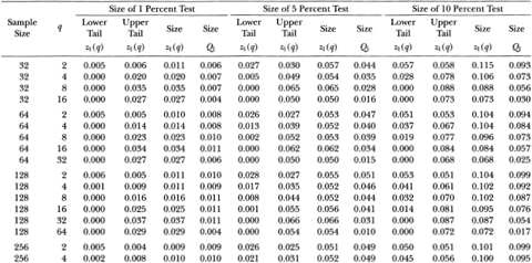
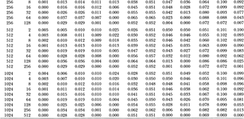
Table 3.1b. Empirical sizes of nominal 1, 5, and 10 percent two-sided variance ratio tests of the random walk null hypothesis with homoskedastic disturbances. The statistic z₂(q) is asymptotically N (O, 1) under the more general conditions of heteroskedastic and weakly dependent (but uncorrelated) random walk increments. The rejection rates for each of the 1, 5, and 10 percent tests are broken down into upper and lower tail rejections to display the skewness of the z₂-statistic's empirical distribution. For comparison, the empirical sizes of the heteroskedasticity-robust one-sided Box-Pierce Q-test (Q₂) using q – 1 autocorrelations are also reported. Each set of rows with a given sample size forms a separate and independent simulation experiment based on 20,000 replications.

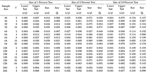
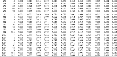
Table 3.1b reports similar results for the heteroskedasticity-robust test statistics z₂(q) and Q₂. For sample sizes greater than 32, the size of the variance ratio test is close to its nominal value when q is small relative to the sample size. As q increases for a given sample, the size increases and then declines, as in Table 3.1a. Again, the variance ratio rejections are primarily due to its upper tail as q increases relative to the sample size. In contrast to the Q₁-test, the heteroskedasticity-robust Box-Pierce test Q₂ increases in size as more autocorrelations are used. For example, in samples of 1024 observations the size of the 5 percent Q₂-test increases from 5.1 to 11.3 percent as q ranges from 2 to 512. In contrast, the size of the variance ratio test starts at 5.2 percent when q = 2, increases to 6.6 percent at q = 256, and falls to 5.8 percent at q = 512.

Tables 3.1a and 3.1b indicate that the empirical size of the variance ratio tests is reasonable even for moderate sample sizes, and is closer to its nominal value than the Box-Pierce tests when the aggregation value becomes large relative to the sample size. However, in such cases most of the variance ratio's rejections are from its upper tail; power considerations will need to be weighed against the variance ratio test's reliability under the null.

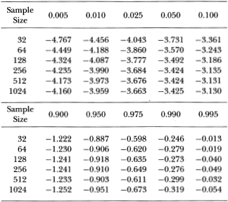
Since the sampling theory for the Q- and z-statistics obtain only asymptotically, the actual size of any test based on these statistics will of course differ from their nominal values in finite samples. Although Tables 3.1a and 3.1b indicate that such differences may not be large for reasonable aggregation values, it may nevertheless seem more desirable to base tests upon the regression t-statistic for which Fuller (1976), Dickey and Fuller (1979, 1981), and Nankervis and Savin (1985) have tabulated the exact finite-sample distribution. Due to the dependence of the t-statistic's distribution on the drift µ, an additional nuisance parameter (a time-trend coefficient) must be estimated to yield a sampling distribution that is independent of the drift. Although it has been demonstrated that the t-statistic from such a regression converges in distribution to that of Dickey and Fuller, there may be some discrepancies in finite samples. Table 3.2 presents the empirical quantiles of the distribution of the t-statistic associated with the hypothesis β = 1 in the regression (3.2.14). A comparison of these quantiles with those given in Fuller (1976, Table 8.5.2) suggests that there may be some significant differences for small samples, but for sample sizes of 500 or greater the quantiles in Table 3.2 are almost identical to those of Dickey and Fuller.

Table 3.2. Empirical quantiles of the (Dickey-Fuller) t-statistic associated with the hypothesis β = 1 in the regression where is IID N (0,1). Each row corresponds to a separate and independent simulation experiment based upon 20,000 replications.

3.3.2 A Heteroshdastic Null Hypothesis

To assess the reliability of the heteroskedasticity-robust statistic z₂(q), we perform simulation experiments under the null hypothesis that the disturbance _t in (3.1) is serially uncorrelated but heteroskedastic in the following manner. Let the random walk disturbance _t satisfy the relation _t ≡ σ_t λ_t, where λ_t is IID N (0, l) and σ_t satisfies

λ_t and ζ_t are assumed to be independent. The empirical studies of French, Schwert, and Starnbaugh (1987) and Poterba and Summers (1986) posit such a process for the variance. Note that σ_t² cannot be interpreted as the unconditional variance of the random walk disturbance _t since σ_t² is itself stochastic and does not correspond to the unconditional expectation of any random variable. Rather, conditional upon σ_t², is normally distributed with expectation 0 and variance σ_t². If, in place of (3.3.1), the variance σ_t² were reparameterized to depend only upon exogenous variables in the time t – 1 information set, this would correspond exactly to Engle's (1982) ARCH process.

The unconditional moments of may be readily deduced by expressing the process explicitly as a function of all the disturbances:

Since σ₀, λ_t and ζ_k are assumed to be mutually independent, it is apparent that is serially uncorrelated at all leads and lags (hence assumption (Al) is satisfied) but is nonstationary and temporally dependent. Moreover, it is evident that for all t and for j ≠ k. Hence assumption (A4) is also satisfied. A straightforward calculation yields the moments of :

From these expressions it is apparent that, for ψ ∈ (0, 1), possesses bounded moments of any order and is unconditionally heteroskedastic; similar calculations for the cross-moments verify assumption (A2). Finally, the following inequality is easily deduced:

Thus assumption (A3) is verified. Note that the kurtosis of is

by Jensen's inequality. This implies that, as for Engle's (1982) stationary ARCH process, the distribution of is more peaked and possesses fatter tails than that of a normal random variate. However, when ψ = 0 or as t increases without bound, the kurtosis of is equal to that of a Gaussian process.

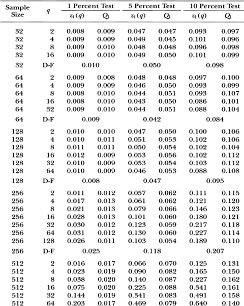
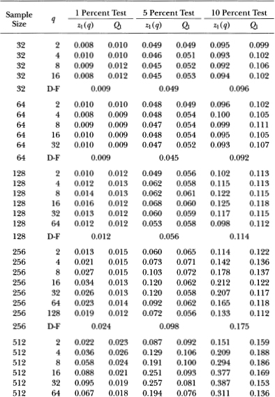
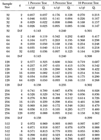
Table 3.3a. Empirical sizes of nominal 1, 5, and 10 percent two-sided variance ratio tests of the random walk null hypothesis with heteroskedastic disturbances. The statistic z₁(q) is asymptotically N (0, 1) under the IID random walk; the z₂(q)-statistic is asymptotically N (0, 1) under the more general conditions of heteroskedastic and weakly dependent (but uncorrelated) increments. For comparison, the empirical sizes of the two-sided Dickey-Fuller t-test (D-F), the one-sided Box-Pierce Q-test (Q₁) and its heteroskedasticity-consistent counterpart (Q₂) (both using q – 1 autocorrelations) are also reported. The specific form of heteroskedasticity is given by . Each set of rows with a given sample size forms a separate and independent simulation experiment based on 20,000 replications.

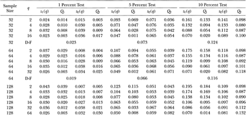
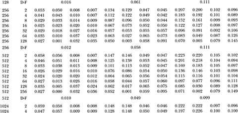
Table 3.3b. Empirical sizes of nominal 1, 5, and 10 percent two-sided variance ratio tests of the random walk null hypothesis with heteroskedastic disturbances. The statistic z₁(q) is asymptotically N (0, 1) under the IID random walk; the z₂(q)-statistic is asymptotically N (0, 1) under the more general conditions of heteroskedastic and weakly dependent (but uncorrelated) increments. For comparison, the empirical sizes of the two-sided Dickey-Fuller t-test (D-F), the one-sided Box-Pierce Q-test (Q₁) and its heteroskedasticity-consistent counterpart (Q₂) (both using q – 1 autocorrelations) are also reported. The specific form of heteroskedasticity is given by . Each set of rows with a given sample size forms a separate and independent simulation experiment based on 20,000 replications.

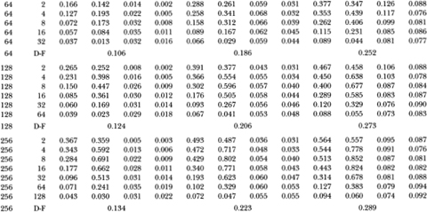
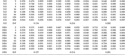
Table 3.3a reports simulation results for the z-, Q-, and Dickey-Fuller t-statistics under the heteroskedastic null hypothesis with parameter ψ = 0.50. It is apparent that both the z₁ and (Q₁-statistics are unreliable in the presence of heteroskedasticity. Even in samples of 512 observations, the empirical size of the 5 percent variance ratio test with q = 2 is 14.7 percent; the corresponding Box-Pierce 5 percent test has an empirical size of 14.6 percent. In contrast, the Dickey-Fuller t-test's empirical size of 4.9 percent is much closer to its nominal value. This is not surprising since Phillips (1987) and Phillips and Perron (1988) have shown that the Dickey-Fuller t-test is robust to heteroskedasticity (and weak dependence) whereas the z₁ and Q₁-statistics are not. However, once the heteroskedasticity-robust z₂ and Q₂-statistics are used, both tests compare favorably with the Dickey-Fuller t-test. In fact, for the more severe case of heterscedasticity considered in Table 3.3b (where ψ = 0.95), the variance ratio and Box-Pierce tests using z₂ and Q₂ are both considerably more reliable than the Dickey-Fuller test.¹⁸ For example, when q/T is ½ in sample sizes of 512 observations, the sizes of 5 percent tests using z₂ and Q₂ are 4.7 and 5.7 percent, respectively; the size of the 5 percent Dickey-Fuller test is 21.6 percent.

3.4 Power

Since a frequent application of the random walk has been in modelling stock market returns, it is natural to examine the power of the variance ratio test against alternative models of asset price behavior. We consider three specific alternative hypotheses. The first two are specifications of the stock price process that have received the most recent attention: the stationary AR(1) process (as in Shiller, 1981; Shiller and Perron, 1985) and the sum of this process and a random walk (as in Fama and French, 1988; Poterba and Summers, 1988).¹⁹ The third alternative is an integrated AR(1) process which is suggested by the empirical evidence in Lo and MacKinlay (1988b).

Before presenting the simulation results, we consider an important limitation of the variance ratio test in Section 3.4.1. In Section 3.4.2 we compare the power of the variance ratio test with that of the Dickey-Fuller and Box-Pierce tests against the stationary AR(1) alternative. Section 3.4.3 reports similar power comparisons for the remaining two alternatives.

3.4.1 The Variance Ratio Test for Large q

Although it will become apparent in Sections 3.4.2 and 3.4.3 that choosing an appropriate aggregation value q for the variance ratio test depends intimately on the alternative hypothesis of interest, several authors have suggested using large values of q generally.²⁰ But because the variance ratio test statistic is bounded below, when q is large relative to T the test may have little power. To see this, let the (asymptotic) variance of the test statistic be denoted by V, where we have from (3.2.6b)

Note that for all natural numbers q, the bracketed function in (3.4.1) is bounded between ½ and 1 and is monotonically increasing in q. Therefore, for fixed n, this implies upper and lower bounds V_U ≡ 4/3n and V_L ≡ 2/3n for the variance V. Since variances must be nonnegative, the lower bound for is –1 (since we have defined to be the variance ratio minus 1). Using these two facts, we have the following lower bound on the (asymptotically) standard normal test statistic :

Note that n is not the sample size (which is given by nq), but is the number of nonoverlapping coarse increments (increments of aggregation value q) available in the sample and is given by T / q.

If q is large relative to the sample size T, this implies a small value for n. For example, if q/T = ½, then the lower bound on the standard normal test statistic z₁(q) is –1.73; the test will never reject draws from the left tail at the 95 percent level of significance!

Of course, there is no corresponding upper bound on the test statistic so in principle it may still reject via draws in the right tail of the distribution. However, for many alternative hypotheses of interest the population values of their variance ratios are less than unity,²¹ implying that for those alternatives rejections are more likely to come from large negative rather than large positive draws of z₁(q). For this reason and because of the unreliability of large-sample theory under the null when q/ T is large, we have chosen q to be no more than one-half the total sample size throughout this study.

3.4.2 Power against a Stationary AR(1) Alternative

As a model of stock market fads, Shiller (1981) has suggested the following AR(1) specification for the log-price process X_t:

where ø is positive and less than unity. To determine the power of the variance ratio test against this alternative, we choose values of the parameters that yield an interesting range of power across sample sizes and aggregation values. Since the power does not depend on a, we set it to zero without loss of generality. Table 3.5a reports the power of the variance ratio, Dickey-Fuller t- and Box-Pierce Q-tests at the 1, 5 and 10 percent levels against the AR(1) alternative with parameters . 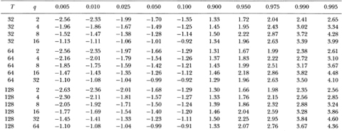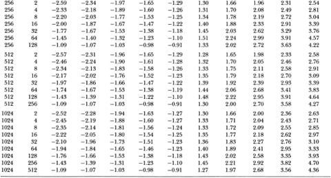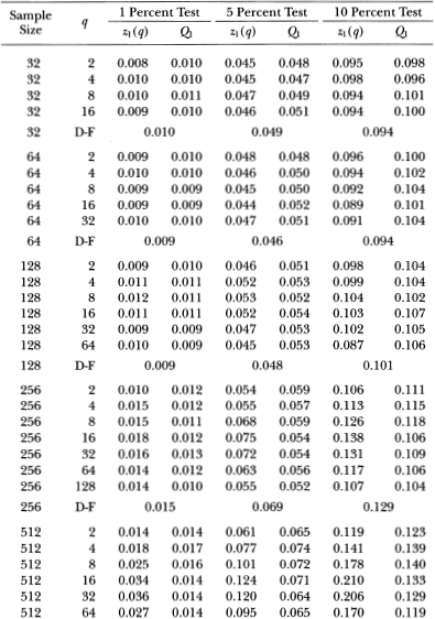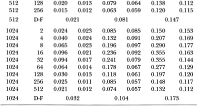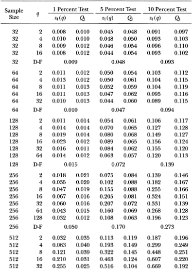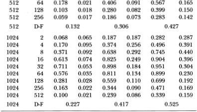The critical values of all three test statistics were empirically determined by simulation under the IID Gaussian null. In the interest of brevity, we report the empirical critical values in Table 3.4 for the variance ratio test only.²²

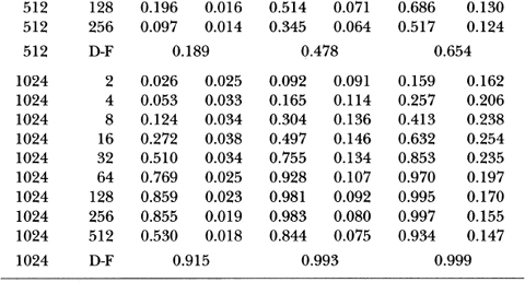
For a fixed number of observations, the power of the variance ratio test first increases and then declines with the aggregation value q. The increase can be considerable; as the case of 1024 observations demonstrates, the power is 9.2 percent when q = 2 but jumps to 98.3 percent when q = 256. The explanation for the increase in power lies in the behavior of the AR(1) alternative over different sampling intervals: the first-order autocorrelation coefficient of AR(1) increments grows in absolute value (becomes more negative) as the increment interval increases. This implies that, although X_t may have a root close to unity (0.96), its first-differences behave less like random walk increments as the time interval of the increments grows. It is therefore easier to detect an AR(1) departure from the random walk by comparing longer first-difference variances to shorter ones, which is precisely what the variance ratio does for larger q. However, as q is increased further the power declines. This may be attributed to the imprecision with which the higher-order autocorrelations are estimated for a fixed sample size. Since the variance ratio with aggregation value q is approximately a linear combination of the first q – 1 autocorrelations, a larger value of q/ T entails estimating higher-order autocorrelations with a fixed sample size. The increased sampling variation of these additional autocorrelations leads to the decline in power.²³

Table 3.4. Empirical quantiles of the (asymptotically) N (0, 1) variance ratio test statistic z₁{q) under simulated IID Gaussian random walk increments, where q is the aggregation value. Each set of rows with a given sample size forms a separate and independent simulation experiment based on 20,000 replications.

Although the most powerful variance ratio test is more powerful than the Dickey-Fuller t-test, the difference is generally not large. However, the variance ratio test clearly dominates the Box-Pierce Q-test. With a sample of 512 observations the power of a 5 percent variance ratio test is 51.4 percent (q = 128) whereas the power of the corresponding Q-test is only 7.1 percent. However, with an aggregation value of q = 2 the variance ratio has comparable power to the Box-Pierce test. Again, this is as expected since they are quite similar statistics when q = 2 (the variance ratio is approximately one plus the first-order autocorrelation coefficient and the Box-Pierce statistic is the first-order autocorrelation squared).

We conclude that, against the stationary AR(1) alternative, the variance ratio test is comparable to the Dickey-Fuller t-test in power and both are considerably more powerful than the Box-Pierce test.

3.4.3 Two Unit Root Alternatives to the Random Walk

Several recent studies have suggested the following specification for the log-price process X_t:

where Y_t is a stationary process and Z_t is a Gaussian random walk independent of Y_t.²⁴ To be specific, let Y_t be an AR(1); thus:

Again, without loss of generality we set α to 0; ρ is set to 0.96; is normalized to unity; and takes on the values 0.50,1.00 and 2.00 so that the conditional variability of the random walk relative to the stationary component is two, one, and one-half, respectively. Tables 3.5b–3.5d report the power of the variance ratio, Dickey-Fuller t and Box-Pierce Q-tests against this alternative.

Table 3.5a. Power of the two-sided variance ratio test (using the z₁(q) statistic) against the stationary AR(1) alternative IID N (0, 1) and ø = 0.96. For comparison, the power of the one-sided Box-Pierce (Q-test (Q₁) and the two-sided Dickey-Fuller t-test (D-F) are also reported. Each set of rows with a given sample size forms a separate and independent simulation experiment based on 20,000 replications.

Note that this specification contains a unit root (it is an ARIMA(1, 1, 1)), and hence, asymptotically, the power of the Dickey-Fuller t-test should equal its size.²⁵ However, since Schwert (1987a,b) has shown the finite-sample behavior of the Dickey-Fuller test to be quite erratic, we report its power for comparison.

Table 3.5b gives the power results for the z₁-, Q₁-, and t-statistics against this ARIMA(1, 1, 1) alternative where the variance of the random walk innovation is twice the variance of the AR(1) disturbance. Although none of the tests are especially powerful under these parameter values, the variance ratio test seems to dominate the other two. For a sample size of 1024, the power of the variance ratio test is 24.1 percent for q = 32 whereas the corresponding power of the Dickey-Fuller and Box-Pierce tests are 10.4 and 7.9 percent, respectively.

Table 3.5b. Power of the two-sided variance ratio test (using the z₁(q)-statistic) against the ARIMA(1, 1, 1) alternative X_t = Y_t + Z_t, where Y_t = 0.96 Y_{t – 1} + , _t IID N (O, 1) and Z_t = + γ_t, γ_t IID N (0, ½). For comparison, the power of the one-sided Box-Pierce Q-test (Q₁) and the two-sided Dickey-Fuller t-test (D-F) are also reported. Each set of rows with a given sample size forms a separate and independent simulation experiment based on 20,000 replications.

As in the case of the stationary AR(1) alternative, the power of the variance ratio test also rises and falls with q against the ARIMA(1, 1, 1) alternative. In addition to the factors discussed in Section 3.4.2, there is an added explanation for this pattern of power. For small to medium differencing intervals the increments of X_t behave much like increments of an AR(1), hence power increases with q in this range. For longer differencing intervals the random walk component dominates. Hence the power declines beyond some aggregation value q.

As the variance of the random walk's disturbance declines relative to the variance of the stationary component's, the power of the variance ratio test increases. Table 3.5c reports power results for the case where the variances of the two components' innovations are equal, and in Table 3.5d the variance of the random walk innovation is half the variance of the AR(1) innovation. In the latter case, the 5 percent variance ratio test has 89.8 percent power for q = 32 and T = 1024 compared to 41.7 percent and 18.4 percent power for the Dickey-Fuller and Box-Pierce tests, respectively. Although the qualitative behavior of the three tests are the same in Tables 3.5b–3.5d, the variance ratio test is considerably more powerful than the other two when the variance of the stationary component is larger than that of the random walk. Moreover, the pattern of power as a function of q clearly demonstrates that against this alternative, it is not optimal to set q as large as possible.²⁶

Table 3.5c. Power of the two-sided variance ratio test (using the z₁(q)-statistic) against the ARIMA(1, 1, 1) alternative X_t = Y_t + Z_t, where Y_t = 0.96 Y_t–1 + , _t IID N (0, 1) and IID N (0, 1). For comparison, the power of the one-sided Box-Pierce Q-test (Q₁) and the two-sided Dickey-Fuller t-test (D-F) are also reported. Each set of rows with a given sample size forms a separate and independent simulation experiment based on 20,000 replications.

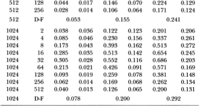
Since both the stationary AR(1) and the AR(1) plus random walk are not empirically supported by Lo and MacKinlay's (1988b) results for weekly stock returns, we consider the power of the variance ratio test against a more relevant alternative hypothesis suggested by their empirical findings: an integrated AR(1), i.e., an ARIMA(1, 1, 0). Specifically, if X_t is the log-price process, then we assume

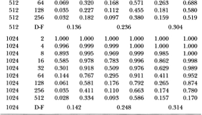
where | k | < 1. Since this alternative obviously possesses a unit root, we expect the standard unit root tests to have poor power against it. Nevertheless for comparison we report the power of the Dickey-Fuller t-test along with the power of the variance ratio and Box-Pierce tests. The parameters are set to (0.20, 1) for all the simulations in Table 3.5e. Unlike its behavior under the stationary AR(1) alternative, against this integrated process the variance ratio's power declines as q increases. With a sample size of 1024, the power of a 5 percent test is 100 percent when q = 2, but falls to 9.3 percent when q = 512. In contrast to the AR(1), the behavior of the integrated process's increments is farthest from a random walk for short differencing intervals (since the increments follow a stationary AR(1) by construction). As the differencing interval increases, the autocorrelation of the increments decreases and it becomes more difficult to distinguish between this process and the random walk.

Table 3.5d. Power of the two-sided variance ratio test (using the z₁(q)-statistic) against the ARIMA(1, 1, 1) alternative , where IID N (0, 1) and IID N (0, 2). For comparison, the power of the one-sided Box-Pierce Q-test (Q₁) and the two-sided Dickey-Fuller t-test (D-F) are also reported. Each set of rows with a given sample size forms a separate and independent simulation experiment based on 20,000 replications.

Observe that for smaller aggregation values the variance ratio test is more powerful than the Q-test, but the Q-test dominates when q is large. This result is due to the fact that the Box-Pierce Q does not distinguish between the upper and lower tails of the null distribution (since Q is the sum of squared autocorrelations) whereas the variance ratio test does.

3.5 Conclusion

Our simulations indicate that the variance ratio test of the random walk hypothesis generally yields reliable inferences under both the IID Gaussian and the heteroskedastic null hypotheses. By selecting the aggregation value q appropriately, the power of the variance ratio test is comparable to that of the Box-Pierce and Dickey-Fuller tests against the stationary AR(1) alternative and is more powerful than either of the two tests against the two unit root alternatives. However, because of the variance ratio's skewed empirical distribution, caution must be exercised when q is large relative to the sample size.

Table 3.5e. Power of the two-sided variance ratio test (using the statistic z₁(q)) against the ARIMA(1, 1, 0) alternative IID N (0, 1), k = 0.20. For comparison, the power of the one-sided Box-Pierce Q-test (Q₁) and the two-sided Dickey-Fuller t-test (D-F) are also reported. Each set of rows with a given sample size forms a separate and independent simulation experiment based on 20,000 replications.

These results emphasize dramatically the obvious fact that the power of any test may differ substantially across alternatives. A sensible testing strategy must consider not only the null hypothesis but also the most relevant alternative. Although the variance ratio test has advantages over other tests under some null and alternative hypotheses, there are of course other situations in which those tests may possess more desirable properties. Nevertheless, the Monte Carlo evidence suggests that the variance ratio test has reasonable power against a wide range of alternative.²⁷ The simplicity, reliability, and flexibility of the variance ratio test make it a valuable tool for inference.

---

¹See, for example, Gould and Nelson (1974), Hall (1978), Lucas (1978), Shiller (1981), Kleidon (1986), and Marsh and Merton (1986).

²See, for example, Campbell and Mankiw (1987), Cochrane (1987b, 1987c), Huizinga (1987), Lo and MacKinlay (1988b), and Poterba and Summers (1988).

³Dickey and Fuller (1979, 1981) make the stronger assumption of independently and identically distributed Gaussian disturbances.

⁴Also, see Cochrane (1987c) who uses this fact to show that trend-stationarity and diierence-stationarity cannot be distinguished with a finite amount of data.

⁵We are grateful to one of the two referees for this insight.

⁶The usual regression t-statistic's limiting distribution depends discontinuously on the presence or absence of a nonzero drift (see Nankervis and Savin, 1985; Perron, 1986). This dependence on the drift may be eliminated by the inclusion of a time trend in the regression, but requires the estimation of an additional parameter and may affect the power of the resulting test. Section 3.4 reports power comparisons.

⁷ The Gaussian assumption may, of course, be weakened considerably. We present results for this simple case only for purposes of comparison to other results in the literature that are derived under identical conditions. In Section 3.2.2 we relax both the independent and the identically distributed assumptions.

⁸Although we have defined the total number of observations T ≡ nq to be divisible by the aggregation value q, this is only for expositional convenience and may be easily generalized.

⁹The use of variance ratios is, of course, not new. Most recently, Campbell and Mankiw (1987), Cochrane (1987b, 1987c), French and Roll (1986) and Huizinga (1987) have all computed variance ratios in a variety of contexts. However, those studies do not provide any formal sampling theory for our statistics. Specifically, Cochrane (1988) and French and Roll (1986) rely upon Monte Carlo simulations to obtain standard errors for their variance ratios under the null. Campbell and Mankiw (1987) and Cochrane (1987~d) o derive the asymptotic variance of the variance ratio, but only under the assumption that the aggregation value q grows with (but more slowly than) the sample size T. Specifically, they use Priestley's (1981, p. 463) expression for the asymptotic variance of the estimator of the spectral density of X_t at frequency zero with a Bartlett window as the appropriate asymptotic variance of the variance ratio. But Priestley's result requires (among other things) that q → ∞, T → ∞, and q/T → 0. In this chapter, we develop the formal sampling theory of the variance ratio statistics for the more general case.

Our variance ratio may, however, be related to the spectral density estimates in the following way. Letting f(0) denote the spectral density of the increments X_t at frequency zero, we have the following relation:

where γ(k) is the autocovariance function. Dividing both sides by the variance γ(0) then yields

where f* is the normalized spectral density and ρ(k) is the autocorrelation function. Now in order to estimate the quantity π f*(0) the infinite sum on the right-hand side of the preceding equation must obviously be truncated. If, in addition to truncation, the autocorrelations are weighted using Newey and West's (1987) procedure, then the resulting estimator is formally equivalent to our statistic. Although he does not explicitly use this variance ratio, Huizinga (1987) does employ the Newey and West (1987) estimator of the normalized spectral density.

¹⁰In addition to admitting heteroskedasticity, it should be emphasized that assumptions (A2) and (A3) also follow for more general heterogeneity and weak dependence. Our reason for focusing on heteroskedasticity is merely its intuitiveness: it is more difficult to produce an interesting example of, for example, an uncorrelated homoskedastic time series which is weakly dependent and heterogeneously distributed.

¹¹Although this assumption may be weakened considerably, it would be at the expense of computational simplicity since in that case the asymptotic covariances of the autocorrelations must be estimated. Specifically, since the variance ratio statistic is asymptotically equivalent to a linear combination of autocorrelations, its asymptotic variance is simply the asymptotic variance of the linear combination of autocorrelations. If (A4) obtains, this variance is equal to the weighted sum of the individual autocorrelation variances. If (A4) is violated, then the autocovariances of the autocorrelations must also be estimated. This is readily accomplished using, for example, the approach in Newey and West (1987). Note that an even more general (and possibly more exact) sampling theory for the variance ratios may be obtained using the results of Dufour and Roy (1985). Again, this would sacrifice much of the simplicity of our asymptotic results.

¹²An equivalent and somewhat more intuitive method of arriving at (3.2.9c) is to consider the regression of the increments X_t on a constant and the jth lagged increment X_t–j. The estimated slope coefficient is then simply the jth autocorrelation coefficient and the estimator δ(j) of its variance is numerically identical to White's (1980) heteroskedasticity-consistent covakance matrix estimator. Note that White (1980) requires independent disturbances, whereas White and Domowitz (1984) allow for weak dependence (of which uncorrelated errors is, under suitable regularity conditions, a special case). Taylor (1984) also obtains this result under the assumption that the multivariate distribution of the sequence of disturbances is symmetric.

¹³Since we include the Box-Pierce test only as an illustrative comparison to the variance ratio test, we have not made any effort to correct for finite-sample biases as in Ljung and Box (1978).

¹⁴Due to the dependence of the t-statistic's distribution on the drift µ, a time trend t must be included in the regression to yield a sampling theory for the t-statistic which is independent of the nuisance parameter.

¹⁵Yet another recent test of the random walk hypothesis is the regression test proposed by Fama and French (1988). Since Monte Carlo experiments by Poterba and Summers (1988) indicate that the variance ratio is more powerful than this regression test against several interesting alternatives, we do not explore its finite-sample properties here.

¹⁶Null simulations were performed in single-precision FORTRAN on a DECVAX 8700 using the random number generator GGNML of the IMSL subroutine library. Power simulations were performed on an IBM 3081 and a VAX 8700 also in single-precision FORTRAN using GGNML.

¹⁷More direct evidence of this skewness is presented in Table 3.4, in which the fiactiles of the variance ratio test statistic are reported. See also the discussion in Section 3.4.1.

¹⁸This provides further support for Schwert's (1987b) finding that, although the Dickey-Fuller distribution is still valid asymptotically for a variety of non-IID disturbances, the t-statistic's rate of convergence may be quite slow.

¹⁹The latter specification is, of course, not original to the financial economics literature but has its roots in Muth (1960) and, more recently, Beveridge and Nelson (1981).

²⁰For example, Campbell and Mankiw's (1987) asymptotic sampling theory requires that q goes to infinity as the sample size T goes to infinity (although q must grow at a slower rate than T). Also, for a sample size of T Huizinga (1987) sets q to T – 1.

²¹For example, as q increases without bound the variance ratio (population value) of increments any stationary process will converge to 0. For the sum of a random walk and an independent stationary process, the variance ratio of its increments will also converge to a quantity less than unity as q approaches infinity.

²²Diebold (1987) tabulates the finite sample distributions of actual variance ratios under many other null hypotheses of interest. Although we have not compared each of our empirical quantiles with his, we have spot-checked several for consistency and have found discrepancies only in the extreme tail areas. For example, with a sample size of 1024 and q = 2, Diebold's implied value for the upper 0.5 percent quantile of our test statistic z₁ is 2.48 (using his Table 16), whereas our value in Table 3.4 is 2.63. There are at least two possible causes for this discrepancy. First, Diebold's results are based on 10,000 replications whereas ours use 20,000. Second, we simulated the bias-corrected statistic whereas Diebold employed the unadjusted variance ratio. For larger tail areas, this discrepancy vanishes.

²³If the variance ratio test were performed using asymptotic critical values against the AR(1) alternative, there is another cause of the power to decline as q increases. Under the AR(1) model, it is apparent that the theoretical values of the variance ratios are all less than unity, implying that the expectations of the z_l-statistics are negative. But it is shown in Section 3.4.1 that the z_l-statistic is bounded below when the asymptotic variance is used to form z_l, and that the lower bound is an increasing function of the ratio of q to the sample size. Therefore, when the deviation of the alternative from the random walk is in the form of negative draws of z_l (as in the AR(1) case), the variance ratio test cannot reject the null hypothesis when q is large relative to the number of observations. This is yet another reason we choose q to be less than or equal to one-half the sample size.

²⁴See, for example, Summers (1986), Fama and French (1988). and Poterba and Summers (1988).

²⁵ To see this, observe that (3.4.4)h as the following ARIMA(1,1,1) representation:

where

²⁶In fact, the q for which the variance test has the most power for a given sample size will depend on the ratio of the stationary component's innovation variance to the variance of the random walk's disturbance. Unfortunately, this fact cannot be observed in our tables because we have set q to be powers of 2 for computational convenience. If the variance ratio test's power were tabulated for q = 2, 3, 4,…, T – 1, it would be apparent that against this ARIMA(l, l, 1) alternative the optimal q changes with the ratio of the innovation invariances of the two components.

²⁷ See Hausman (1988) for further evidence of this.