7

Multifactor Models Do Not Explain Deviations from the CAPM

7.1 Introduction

ONE OF THE IMPORTANT PROBLEMS of modern financial economics is the quantification of the tradeoff between risk and expected return. Although common sense suggests that investments free of risk will generally yield lower returns than riskier investments such as the stock market, it was only with the development of the Sharpe-Lintner capital asset pricing model (CAPM) that economists were able to quantify these differences in returns. In particular, the CAPM shows that the cross-section of expected excess returns of financial assets must be linearly related to the market betas, with an intercept of zero. Because of the practical importance of this risk-return relation, it has been empirically examined in numerous studies. Over the past fifteen years, a number of studies have presented evidence that contradict the CAPM, statistically rejecting the hypothesis that the intercept of a regression of excess returns on the excess return of the market is zero.

The apparent violations of the CAPM have spawned research into possible explanations. In this chapter, the explanations will be divided into two categories: risk-based alternatives and nonrisk-based alternatives. The risk-based category includes multifactor asset pricing models developed under the assumptions of investor rationality and perfect capital markets. For this category, the source of deviations from the CAPM is either missing risk factors or the misidentification of the market portfolio as in Roll (1977).

The nonrisk-based category includes biases introduced in the empirical methodology, the existence of market frictions, or explanations arising from the presence of irrational investors. Examples are data-snooping biases, biases in computing returns, transaction costs and liquidity effects, and market inefficiencies. Although some of these explanations contain elements of risk, the elements of risk are different than those associated with perfect capital markets.

The empirical finding that the intercepts of the CAPM deviate statistically from zero has naturally led to the empirical examination of multifactor asset pricing models motivated by the arbitrage pricing theory (APT) developed by Ross (1976) and the intertemporal capital asset pricing model (IGAPM) developed by Merton (1973) (see Fama, 1993, for a detailed discussion of these multifactor model theories). The basic approach has been to introduce additional factors in the form of excess returns on traded portfolios and then reexamine the zero-intercept hypothesis. Fama and French (1993) use this approach and document that the estimates of the CAPM intercepts deviate from zero for portfolios formed on the basis of the ratio of book value to market value of equity as well as for portfolios formed based on market capitalization.¹ On finding that the intercepts for these portfolios with a three-factor model are closer to zero, they conclude that missing risk factors in the CAPM are the source of the deviations. They go on to advocate the use of a multifactor model, stating that, with respect to the use of the Sharpe-Lintner CAPM, their results “should help to break this common habit” (p. 44).

However, the conclusion that additional risk factors are required may be premature. One of several explanations consistent with the presence of deviations is data-snooping, as presented in Lo and MacKinlay (1990). The argument is that on an ex post basis one will always be able to find deviations from the CAPM . Such deviations considered in a group will appear statistically significant. However, they are merely a result of grouping assets with common disturbance terms. Since in financial economics our empirical analysis is ex post in nature, this problem is difficult to control. Direct adjustments for potential snooping are difficult to implement and, when implemented, make it very difficult to find real deviations.

While it is generally difficult to quantify and adjust for the effects of data-snooping biases, there are some related biases that can be examined. One such case pursued by Kothari, Shanken, and Sloan (1995) is sample selection bias. The authors show that significant biases can arise in academic research when the analysis is conditioned on the assets appearing in both the Center for Research in Security Prices (CRSP) database and the Compustat database. Their analysis suggests that deviations from the CAPM such as those documented by Fama and French (1993) can be explained by sample selection biases. Breen and Korsyczyk (1993) provide further evidence on selection biases that supports the Kothari, Shanken, and Sloan conclusion.

Other researchers interpret the deviations from the CAPM as indications of the presence of irrational behavior by market participants (e.g., DeBondt and Thaler, 1985). A number of theories have been developed that are consistent with this line of thought. A recent example is the work of Lakonishok, Shleifer, and Vishny (1994) who argue that the deviations arise from investors following naive strategies, such as extrapolating past growth rates too far into the future, assuming a trend in stock prices, overreacting to good or bad news, or preferring to invest in firms with a high level of profitability. With this alternative the possibility of nonzero intercepts arises not only from missing risk factors but also from specific firm characteristics.

Conrad and Kaul (1993) consider the possibility that biases in computed returns explain the deviations. They find that the implicit portfolio rebalancing in most analyses biases measured returns upwards, leading to overstated returns and CAPM deviations. This problem will be most severe for tests using frequently rebalanced portfolios and short observation intervals.

Finally, market frictions and liquidity effects could induce a nonzero intercept in the CAPM tests. Since the model is developed in a perfect market, such effects are not accommodated. Amihud and Mendelson (1986) present some evidence of returns containing effects from market frictions and demands for liquidity.

The controversy over whether or not the CAPM deviations are due to missing risk factors flourishes because empirically it is hard to distinguish between the various hypotheses. On an ex post basis, one can always find a set of risk factors that will make the asset pricing model intercept zero. Without a specific theory identifying the risk factors, one will always be able to explain the cross-section of expected returns with a multifactor asset pricing model, even if the real explanation lies in one of the nonrisk-based categories.

Although it is difficult to distinguish between the risk-based and nonrisk-based categories, the practical implications of the distinction are important. For example, if the risk-based explanation is correct, then cost of capital calculations using the CAPM can be badly misspecified. A better approach would be to use a multifactor model that captures the missing risk factors. On the other hand, if the deviations are a result of the nonrisk-based explanations, then disposing of the CAPM in favor of a multifactor model may lead to serious errors. The cost of capital estimate from a multifactor model can be very different than the estimate from the CAPM .

In this chapter, we discriminate between the risk-based and the nonrisk-based explanations using ex ante analysis. The objective is to evaluate the plausibility of the argument that the deviations from the CAPM can be explained by additional risk factors. We argue that one should expect ex ante that CAPM deviations due to missing risk factors will be very difficult to detect because the deviation in expected return is also accompanied by increased variance. We formally analyze the issue using mean-variance efficient set mathematics in conjunction with the zero-intercept F-test presented in Gibbons, Ross, and Shanken (1989) and MacKinlay (1987). The difficulty exists because when deviations from the CAPM or other multifactor pricing models are the result of omitted risk factors, there is an upper limit on the distance between the null distribution of the test statistic and the alternative distribution. With the nonrisk-based alternatives, for which the source of the deviations is something other than missing factors, no such limit exists because the deviations need not be linked to the variances and covariances.

The chapter also draws on a related distinction between the two categories, namely the difference in the behavior of the maximum squared Sharpe measure as the cross-section of securities is increased. (The Sharpe measure is the ratio of the mean excess return to the standard deviation of the excess return.) For the risk-based alternatives the maximum squared Sharpe measure is bounded, and for the nonrisk-based alternatives the maximum squared Sharpe measure is a less useful construct and can, in principle, be unbounded.

The results of the chapter underscore the important role that economic analysis plays in distinguishing among different pricing models for the relation between risk and return. In the absence of specific alternative theories, and without very long time series of data, one is limited in what can be said about risk-return relations among financial securities.

The chapter proceeds as follows. In Section 2 the framework for the analysis is presented and the optimal orthogonal portfolio is defined. This portfolio will play a key role in the arguments of the chapter. Many of the results in the chapter can be related to the values of the squared Sharpe measure for relevant portfolios. In Section 3 the relations between the parameters of the returns and the Sharpe measures are presented. Section 4 develops the implications relating to the controversy over missing risk factors. Theoretically, the framework used to distinguish between risk-based and nonrisk-based explanations assumes a large number of assets. Section 5 illustrates that the usefulness of the framework does not depend on this assumption. The chapter concludes with Section 6.

7.2 Linear Pricing Models, Mean-Variance Analysis, and the Optimal Orthogonal Portfolio

We begin by specifying the distributional properties of excess returns for primary assets in the economy. Let z_t represent the × 1 vector of excess returns for period t. Assume z_t is stationary and ergodic with mean µ and a covariance matrix V that is full rank. Given these assumptions for any set of factor portfolios, a linear relation between the excess returns and the portfolios' excess returns results. The relation can be expressed as

B is the × K matrix of factor loadings, Zp_t is the K × 1 vector of time- t factor portfolio excess returns, andα and ε_t are × 1 vectors of asset return intercepts and disturbances, respectively. The values of α, B, and Σ) will depend on the factor portfolios. This dependence is suppressed for notational convenience.

It is well-known that all of the elements of the vector α will be zero if a linear combination of the factor portfolios forms the tangency portfolio (i.e., the mean-variance efficient portfolio of risky assets given the presence of a risk-free asset). Let z_qt be the excess return of the (ex ante) tangency portfolio and let x_q be the × 1 vector of portfolio weights. Here, and throughout the chapter, let represent a conforming vector of ones. From mean-variance analysis:

In the context of our previous discussion, the asset pricing model will be considered well-specified when the tangency portfolio can be formed from a linear combination of the K-factor portfolios.

Our interest is in formally developing the relation between the deviations from the asset pricing model, α, and the residual covariance matrix Σ when a linear combination of the factor portfolios does not form the tangency portfolio. To facilitate this we define the optimal orthogonal portfolio,² which is the unique portfolio given assets that can be combined with the factor portfolios to form the tangency portfolio and is orthogonal to the factor portfolios.

Take as given K-factor portfolios which cannot be combined to form the tangency portfolio or the global minimum variance portfolio. A portfolio h will be defined as the optimal orthogonal portfolio with respect to these K-factor portfolios if

for a K × 1 vector ω, where Xp is the × K matrix of asset weights for the factor portfolios, X_h is the × 1 vector of asset weights for the optimal orthogonal portfolio, and x_q is the × 1 vector of asset weights for the tangency portfolio. If one considers a model without any factor portfolios (K = 0), then the optimal orthogonal portfolio will be the tangency portfolio.

The weights of portfolio h can be expressed in terms of the parameters of the K-factor model. For the vector of weights,

where the † superscript indicates the generalized inverse. The usefulness of this portfolio comes from the fact that when added to (7.2.1) the intercept will vanish and the factor-loading matrix B will not be altered. The optimality restriction in (7.2.7) leads to the intercept vanishing, and the orthogonality condition in (7.2.8) leads to B being unchanged. Adding in Z_ht:

The link results from comparing (7.2.1) and (7.2.10). Taking the unconditional expectations of both sides,

and by equating the variance of with the variance of β_hZ_ht + u_t:

The key link between the model deviations and the residual variances and covariances emerges from (7.2.17). The intuition for the link is straightforward. Deviations from the model must be accompanied by a common component in the residual variance to prevent the formation of a portfolio with a positive deviation and a residual variance that decreases to zero as the number of securities in the portfolio grows. When the link is not present (i.e., the link is undone by ), asymptotic arbitrage opportunities will exist.

7.3 Squared Sharpe Measures

The squared Sharpe measure is a useful construct for interpreting much of the ensuing analysis. The Sharpe measure for a given portfolio is calculated by dividing the mean excess return by the standard deviation of return. It is well-known that the tangency portfolio q will have the maximum squared Sharpe measure of all portfolios.³ The squared Sharpe measure of q, , is

Since the K-factor portfolios and the optimal orthogonal portfolio h can be combined to form the tangency portfolio, it follows that the maximum squared Sharpe measure of these K + 1 portfolios will be . Since h is orthogonal to the portfolios , one can express as the sum of the squared Sharpe measure of the orthogonal portfolio and the squared maximum Sharpe measure of the factor portfolios,

where

In applications we will be employing subsets of the assets. The factor portfolios need not be linear combinations of the subset of assets. Results similar to those above will hold within a subset of N assets. For the subset analysis when considering the tangency portfolio (of the subset), the maximum squared Sharpe measure of the assets and factor portfolios, and the optimal orthogonal portfolio for the subset, it is necessary to augment the N assets with the factor portfolios . Defining as the N + K × 1 vector with mean and covariance matrix V^*_s, for the tangency portfolio of these N + K assets:

The subscript s indicates that a subset of the assets is being considered. If any combination of the factor portfolios is a linear combination of the N assets, it will be necessary to use the generalized inverse in (7.3.3).

As we shall see, the analysis (with a subset of assets) will involve the quadratic computed using the parameters for the N assets. Gibbons, Ross, and Shanken (1989) and Lehmann (1988, 1992) provide interpretations of this quadratic term in terms of Sharpe measures. Assuming Σ

is of full rank (if Σ is singular then one must use the generalized inverse), they show

Consistent with (7.3.2), for the subset of assets will be the squared Sharpe measure of the subset's optimal orthogonal portfolio h_s. Therefore, for a given subset of assets:

Also note that the squared Sharpe measure of the subset's optimal orthogonal portfolio is less than or equal to that of the population optimal orthogonal portfolio:

Next we use the optimal orthogonal portfolio and the Sharpe measure results together with the model deviation residual variance link to develop implications for distinguishing among asset pricing models. Hereafter we will suppress the s subscript. No ambiguity will result since, in the subsequent analysis, we will be working only with subsets of the assets.

7.4 Implications for Risk-Based Versus Nonrisk-Based Alternatives

Many asset pricing model tests involve testing the null hypothesis that the model intercept is zero using tests in the spirit of the zero-intercept F-test.⁴ A common conclusion is that rejection of this hypothesis using one or more factor portfolios shows that more risk factors are required to explain the risk-return relation, leading to the inclusion of additional factors so that the null hypothesis will be accepted (Fama and French, 1993, adopt this approach). A shortcoming of this approach is that there are multiple potential interpretations of why the hypothesis is accepted. One view is that genuine progress in terms of identifying the “right” asset pricing model has been made. However, the apparent success in identifying a better model may also have come from finding a good within-sample fit through data-snooping. The likelihood of this possibility is increased by the fact that the additional factors lack theoretical motivation.

This section integrates the link between the pricing model intercept and the residual covariance matrix of (7.2.17) and the squared Sharpe measure results with the distribution theory for the zero-intercept F-test to discriminate between the two interpretations. We consider two approaches. The first approach is a testing approach that compares the null hypothesis test statistic distribution with the distribution under each of the alternatives. The second approach is estimation-based, drawing on the squared Sharpe measure analysis to develop estimators for the squared Sharpe measure of the optimal orthgonal portfolio. Before presenting the two approaches, the zero-intercept F-test is summarized.

7.4.1 Zero Intercept F-Test

To implement the F-test, the additional assumption that excess asset returns are jointly normal and temporally independently and identically distributed is added. This assumption, though restrictive, buys us exact finite sample distributional results, thereby simplifying the analysis. However, it is important to note that this assumption is not central to the point; similar results will hold under much weaker assumptions. Using a generalized method of moments approach, MacKinlay and Richardson (1991) present a more general test statistic that has asymptotically a chi-square distribution. Analysis similar to that presented for the F-test holds for this general statistic.

We begin with a summary of the zero-intercept F-test of the null hypothesis that the intercept vector α from (7.2.1) is zero. Let H₀ be the null hypothesis and H_a be the alternative:

H_o can be tested using the following test statistic:

where T is the number of time series observations, N is the number of assets or portfolios of assets included, and K is the number of factor portfolios. The hat superscripts indicate the maximum likelihood estimators. Under the null hypothesis, θ₁ is unconditionally distributed central F with N degrees of freedom in the numerator and T – N – K degrees of freedom in the denominator.

The distribution of θ₁ can also be characterized in general. Conditional on the factor portfolio excess returns, the distribution of θ₁ is

where λ is the noncentrality parameter of the F distribution. If K = 0, then the term will not appear in (7.4.3) or in (7.4.5) and θ₁ will be unconditionally distributed noncentral F.

7.4.2 Testing Approach

In this approach we consider the distribution of θ₁ under two different alternatives. The alternatives can be separated by their implications for the maximum value of the squared Sharpe measure. With the risk-based multifactor alternative there will be an upper bound on the squared Sharpe measure, whereas with the nonrisk-based alternatives the maximum squared Sharpe measure can be unbounded (as the number of assets increases).

First we consider the distribution of θ₁ under the alternative hypothesis when deviations are due to missing factors. Drawing on the results for the squared Sharpe measures, the noncentrality parameter of the F distribution is

From (7.3.7), the third term in (7.4.6) is positive and bounded above by . The second term is bounded between zero and one. Thus there is an upper bound for λ,

The second inequality follows from the fact that the tangency portfolio q has the maximum Sharpe measure of any asset or portfolio.⁵

Given a maximum value for the squared Sharpe measure, the upper bound on the noncentrality parameter can be important. With this bound, independent of how one arranges the assets to be included as dependent variables in the pricing model regression and for any value of N, there is a limit on the distance between the null distribution and the distribution when the alternative is missing factors. (In practice, when using the F-test it will be necessary for N to be less than T –K so that will be of full rank.) All the assets can be mispriced and yet the bound will still apply. As a consequence, one should be cautious in interpreting rejections of the zero intercept as evidence in favor of a model with more risk factors.

In contrast, when the source of nonzero intercepts is nonrisk-based, such as data-snooping, market frictions, or market irrationalities, the notion of a maximum squared Sharpe measure is not useful. The squared Sharpe measure (and the noncentrality parameter) are in principle unbounded because the argument linking the deviations and the residual variances and covariances does not apply. When comparing alternatives with the intercepts of about the same magnitude, in general, one would expect to see larger test statistics in this nonrisk-based case.

One can examine the potential usefulness of the above analysis by considering alternatives with realistic parameter values. We construct the distribution of the test statistic for three cases: the null hypothesis, the missing risk factors alternative, and the nonrisk-based alternative. For the risk-based alternative, we draw on a framework designed to be similar to that in Fama and French (1993). For the nonrisk-based alternative we use a setup that is consistent with the analysis of Lo and MacKinlay (1990) and the work of Lakonishok, Shleifer, and Vishny (1994).

Consider a one-factor asset pricing model using a time series of the excess returns for 32 portfolios for the dependent variable. The one factor (independent variable) is the excess return of the market so that the zero-intercept null hypothesis is the CAPM . The length of the time series is 342 months. This setup corresponds to that of Fama and French (1993, Table 9, regression ii). The null distribution of the test statistic θ₁ is

To define the distribution of θ₁ under the risk-based and nonrisk-based alternatives one needs to specify the parameters necessary to calculate the noncentrality parameter. For the risk-based alternative, given a value for the squared Sharpe measure of the optimal orthogonal portfolio, the distribution corresponding to the upper bound of the noncentrality parameter from (7.4.7) can be considered. The Sharpe measure of the optimal orthogonal portfolio can be obtained using (7.3.2) given the squared Sharpe measures of the tangency portfolio and of the included factor portfolio. Our view is that in a perfect capital markets setting, a reasonable value for the squared Sharpe measure of the tangency portfolio for an observation interval of one month is 0.031 (or approximately 0.6 for the Sharpe measure on an annualized basis). This value, for example, corresponds to a portfolio with an annual expected excess return of 10% and a standard deviation of 16%. If the maximum squared Sharpe measure of the included factor portfolios is the ex post squared Sharpe measure of the CRSP value-weighted index, the implied maximum squared Sharpe measure for the optimal orthogonal portfolio is 0.021. This monthly value of 0.021 would be consistent with a portfolio which has an annualized mean excess return of 8% and annualized standard deviation of 16%.

The selection of the above Sharpe measure can be rationalized both theoretically and empirically. For theoretical justification we consider Sharpe measures of equity returns in the literature examining the equity risk premium puzzle (see Mehra and Prescott, 1985). While the focus of this research does not concern the Sharpe measure, that measure can be calculated from the analysis provided by Cecchetti and Mark (1990) and Kandel and Stambaugh (1991). Both papers are informative for the question at hand since they do not assume any imperfections in the asset markets. If their models, with reasonable parameters, imply Sharpe measures that are higher than the value selected for use in this chapter, the value selected here should perhaps be reconsidered. However, one should not completely rely on the measures from these papers for justification. In the presented models the aggregate equity portfolio generally will not be mean-variance efficient and therefore need not have the highest Sharpe measure of all equity portfolios.

Common to the papers is the use of a representative agent framework and a Markov switching model for the consumption process. The parameters of the consumption process are chosen to match estimates from the data. Cecchetti and Mark, using the standard time-separable constant relative risk aversion utility function, specify a range of values for the time preference parameter and the risk aversion coefficient. For each pair of values they generate the implied theoretical unconditional mean and standard deviation of the equity risk premium from which the Sharpe measures can be calculated. The annualized Sharpe measures range from 0.08 to 0.16, substantially below the value of 0.60 suggested above.

Kandel and Stambaugh allow for more general preferences. For the representative agent, a class is used that allows separation of the effects of risk aversion and intertemporal substitution. The standard time-separable model is a special case with the elasticity of intertemporal substitution equal to the inverse of the risk aversion coefficient. They set the monthly rate of time preference at 0.9978 and consider 16 pairs of the risk aversion coefficient and the intertemporal substitution parameter. The risk aversion coefficient varies from ½ to 29 and the intertemporal substitution parameter varies from to 2. For thirteen of the sixteen cases the annual Sharpe measure of equity is less than 0.6. The three cases where the Sharpe measure is greater than 0.6 seem implausible since they imply the equity risk premium and the interest rate have almost the same variance, an impliciation which is strongly contradicted by historical data. These are the cases with high values for both the risk aversion parameter and the intertemporal substitution parameter. In aggregate, the results in these papers are consistent with the value specified for the maximum squared Sharpe measure in the context of frictionless asset markets.

One can also ask what Sharpe measure is empirically reasonable. To do this, we present historical Sharpe measures for a number of broad-based indices. These measures, some of which represent portfolios actually held, are reported in Table 7.1. For each index, the ex post measure (based on maximum likelihood estimates) and an unbiased squared Sharpe measure estimate are presented. For the July 1963 through December 1991 period the squared Sharpe measures are presented for the CRSP value-weighted index, the CRSP small-stock (10th decile) portfolio, and the ex post optimal portfolio of these two indices plus the long-term government index and the corporate bond index distributed by CRSP in the stock, bonds, bills, and inflation file. The small-stock portfolio has a monthly squared Sharpe measure of0.014(or0.010 using the unbiased estimate), substantially below the value we use for the tangency portfolio. The ex post optimal four-index portfolio's measure is only slightly higher at 0.015.

Table 7.1. Historical Sharpe measures for selected stock indices, where the Sharpe measure is defined as the ratio of the mean excess return to the standard deviation of the excess return. is the monthly ex post squared Sharpe measure and (ann) is the positive square root of this measure annualized. is an unbiased estimate of the monthly squared Sharpe measure and (ann) is the positive square root of this measure annualized. The CRSP value-weighted index is a value-weighted portfolio of all NYSE and Amex stocks. The CRSP small-stock portfolio is the value-weighted portfolio of stocks in the lowest joint NYSE-Amex market value decile. The portfolio of four indices is the portfolio with the maximum ex post squared Sharpe measure. The four indices are the CRSP value-weighted index, the CRSP small-stock decile, the CRSP long-term government bond index, and the CRSP corporate bond index. The bond indices are from the CRSP SBBI file. The 500 index is a value-weighted index of500 stocks. The -Barra value index is an index of stocks within the 500 universe with low ratios of price per share to book value per share. Every six months a breakpoint price-to-book-value ratio is determined so that approximately half the market capitalization of the 500 is below the breakpoint and the other half is above. The value index is a value-weighted index of those stocks in the group of low price-to-book-value ratios. The 500-Barra growth index is an index of stocks within the 500 universe with high price-to-book-value ratios. The growth index is a value-weighted index of those 500 stocks in the group of high price-to-book-value ratios.

Table 7.1 also contains results for the period from January 1981 through June 1992 for the S&P 500 Index, a value index, and a growth index. The value index contains the S&P 500 stocks with low price-to-book-value ratios and the growth index is constructed from stocks with high price-to-book-value ratios. The source of the index return statistics used to calculate the measures is Capaul, Rowley, and Sharpe (1993). These results provide a useful perspective on the maximum magnitudes of Sharpe measures since it is generally acknowledged that the 1980s was a period of strong stock market performance, especially for value-based investment strategies. Given this characterization, one would expect these results to provide a high estimate of possible Sharpe measures. The Sharpe measures from this period are in line with (and lower than) the value used in the analysis of the risk-based alternative. The highest ex post estimate is 0.021 for the value index. Generally, we interpret the evidence in this table as supporting the measure selected to calibrate the analysis for the risk-based alternative.

Proceeding using a squared Sharpe measure of 0.021 for the optimal orthogonal portfolio to calculate λ, the distribution of θ₁ is

This distribution will be used to characterize the risk-based alternative.

We specify the distribution for two nonrisk-based alternatives by specifying values of α, Σ and , and then calculating λ from (7.4.5). To specify the intercepts we assume that the elements of a are normally distributed with a mean of zero. We consider two values for the standard deviation, 0.0007 and 0.001. When the standard deviation of the elements of of is 0.001 about 95% of the alphas will lie between −0.002 and +0.002, an annualized spread of about 4.8%. A standard deviation of 0.0007 for the alphas would correspond to an annual spread of about 3.4%. These spreads are consistent with spreads that could arise from data-snooping⁶ and are also plausible and even somewhat conservative given the contrarian strategy returns presented in Lakonishok, Shleifer, and Vishny. For Σ we use a sample estimate based on portfolios sorted by market capitalization for the period 1963 to 1991 (inclusive). The effect of on λ will typically be small, so we set it to zero. To get an idea of a reasonable value for the non-centrality parameter given this alternative, we calculate the expected value of λ given the distributional assumption for the elements of a conditional upon Σ = . The expected value of the noncentrality parameter is 39.4 for a standard deviation of 0.0007 and 80.3 for a standard deviation of 0.001. Using these values for the noncentrality parameter, the distribution of θ₁ is

A plot of the four distributions from (7.4.8), (7.4.9), (7.4.10), and (7.4.11) is in Figure 7.1. The vertical bar on the plot represents the value

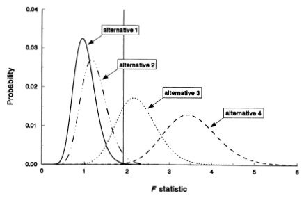
Figure 7.1. Distributions for the CAPM zero-intercept test statistic forfour alternatives. Alternative 1 is the CAPM (null hypothesis); alternative 2 is the risk-based alternative (deviations from the CAPM are from missing risk factors); alternatives 3 and 4 are the nonrisk-based alternative (deviations from the CAPM are unrelated to risk). The distributions are F_32,309 (0), F_32,309 (7.1), F_32,309, (39.4) and F_32,309 (80.3) for alternatives 1, 2, 3, and 4, respectively. The degrees of freedom are set to correspond to monthly observations from July 1963 to December 1992 (342 observations). Using 25 stock portfolios and 7 bond portfolios, and the CRSP value-weighted index as proxy for the market portfolio, the test statistic is 1.91, represented by the vertical line. The probability is calculated using an interval width of 0.02.

1.91 which Fama and French calculate for the test statistic. From this figure notice that the null hypothesis distribution and the risk-based alternative distribution are quite close together, reflecting the impact of the upper bound on the noncentrality parameter (see MacKinlay, 1987, for detailed analysis of this alternative). In contrast, the nonrisk-based alternatives' distributions are far to the right of the other two distributions, consistent with the noncentrality parameter being unbounded for these alternatives.

What do we learn from this plot? First, if the objective is to distinguish among risk-based linear asset pricing models, the zero-intercept test is not particularly useful because the null distribution and the alternative distribution have substantial overlap. Second, if the goal is to compare a risk-based pricing model with a nonrisk-based alternative, the zero-intercept test can be very useful since the distributions of the test statistic for these alternatives have little overlap. Likelihood analysis provides another interpretation of the plot. Specifically, one can compare the values of the densities for the four alternatives at θ₁ = 1.91. Such a comparison leads to the conclusion that the first nonrisk-based alternative is much more likely than the other three.

This analysis can be related to the Fama and French (1993) finding that a model with three factors does a good job in explaining the cross-section of expected returns. For a given finite cross-section under any alternative, the inclusion of the optimal orthogonal portfolio will lead to their result. As a consequence, their result on its own does not support the risk-based category. Indeed, the Fama and French approach to building the extra factors will tend to create a portfolio like the optimal orthogonal portfolio independent of the explanation for the CAPM deviations. Their extra factors essentially assign positive weights to the high positive alpha stocks and negative weights to the large negative alpha stocks. This procedure is likely to lead to a portfolio similar to the optimal orthogonal portfolio because the extreme alpha assets are likely to have the largest (in magnitude) weights in the optimal orthogonal portfolio (since its weights are proportional to Σ^†α; see (7.2.9) ). Further, the fact that when Fama and French increase the number of factors to three the significance of the test statistic only decreases marginally is also consistent with the argument that missing risk factors are not the whole story.

More evidence of the potential importance of nonrisk explanations can be constructed using weekly data. To see why the analysis of weekly data can be informative, consider the biases introduced with market frictions such as the bid-ask spread. Blume and Stambaugh (1983) show that in the presence of the bid–ask bounce, there is an upward bias in observed returns. For asset i and time period t, Blume and Stambaugh show the following approximation for the relation between expected observed returns and expected true returns:

where the superscript “o” distinguishes the returns observed with bid-ask bounce contamination from the true returns; υ_t is the bias which is equal to one-fourth of the proportional bid–ask spread squared. The bias will carry over into the intercept of any factor model. Consider a one-factor model in which the factor is ex ante the tangency portfolio. In this model the intercept for all true asset returns will be zero. However, the intercepts for the observed returns and the squared Sharpe measure of the optimal orthogonal portfolio will be nonzero. If the bias of the observed factor return is zero and if the factor return is uncorrelated with the bid–ask bounce process, then the intercept of the observed returns is

since α_i of the true return will be zero. Then, the squared Sharpe measure of the optimal orthogonal portfolio is

where Σ^o is the residual covariance matrix for the weekly observed returns and υ is the vector of biases for the included portfolios.⁷ When the null hypothesis that the intercepts are zero is examined using observed returns, violations exist solely due to the presence of the bid–ask spread.

Bias of the type induced by the bid–ask spread is interesting because its magnitude does not depend on the length of the observation interval. As a consequence its effect will statistically be more pronounced with shorter observation intervals when the variance of the true returns is smaller. To examine the potential relevance of the above example, the F-test statistic is calculated using a sample of weekly returns for 32 portfolios. The data extends from July 1962 through December 1992 (1,591 weeks). NYSE and Amex stocks are allocated to the portfolios based on beginning-of-year market capitalization. Each portfolio is allocated an equal number of stocks and the portfolios are equal-weighted with rebalancing each week. For these portfolios, using the CRSP value-weighted index as the one factor, the F-test statistic is 2.82. Under the null hypothesis, this statistic has a central F distribution with 32 degrees of freedom in the numerator and 1,558 degrees of freedom in the denominator. (Diagnostics reveal some serial correlation in the residuals of the weekly one-factor model, in which case the null distribution will not be exactly central F.) This statistic can be cast in terms of the alternatives presented in Figure 7.1 since the noncentrality parameter of the F distribution will be approximately invariant to the observation interval and hence only the degrees of freedom need to be adjusted. Figure 7.2 presents the results that correspond to the weekly observation interval. Basically, these results reinforce the monthly observation results in that the observed statistic is most consistent with the nonrisk-based category.

In summary, the results suggest that the risk-based missing risk factors argument is not the whole story. Figures 7.1 and 7.2 show that the test statistic is still in the upper tail when the distribution of θ₁ in the presence of missing risk factors is tabulated. The p-value using this distribution is 0.03 for the monthly data and less than 0.001 for weekly data. Hence there is a lack of support for the view that missing factors completely explain the deviations.

On the other hand, given the parametrizations considered, there is some support for the nonrisk-based alternative views. The test statistic falls

Figure 7.2. Distributions for the CAPM zero-intercept test statistic forfour alternatives. Alternative 1 is the CAPM (null hypothesis); alternative 2 is the risk-based alternative (deviations from the CAPM are from missing risk factors); alternatives 3 and 4 are the nonrisk-based alternative (deviations from the CAPM are unrelated to risk). The distributions are F_32,1558 (0,) F_32,1558 (7.1), F_32,1558 (39.4), and F_32,1558 (80.3) for alternatives 1, 2; 3, and 4, respectively. The degrees of freedom are set to correspond to weekly observations from fuly 1962 to December 1992 (1,591 observations). Using 32 stock portfolios and the CRSP value-weighted index as a proxy for the market portfolio, the test statistic is 2.82, represented by the vertical line. The probability is calculated using an interval width of 0.02.

almost in the middle of the nonrisk-based alternative with the lower standard deviation of the elements of alpha. Several of the nonrisk-based alternatives could equally well explain the results. Different nonrisk-based views can give the same noncentrality parameter and test statistic distribution. The results are consistent with the data-snooping alternative of Lo and MacKinlay (1990), the related sample selection biases discussed by Kothari, Shanken, and Sloan (1995) and Breen and Korajczyk (1993), and the presence of market inefficiencies. The analysis suggests that missing risk factors alone cannot explain the empirical results.

7.4.3 Estimation Approach

In this section we present an estimation approach to make inferences about possible values for Sharpe measures. An estimator for the squared Sharpe measure of the optimal orthogonal portfolio for a given subset of assets is employed. Using this estimator and its variance, confidence intervals for the squared Sharpe measure can be constructed, facilitating judgments on the question of the value implied by the data and reasonable alternatives given this value. An unbiased estimator of the squared Sharpe measure is presented. This estimator corrects for the bias that is introduced by searching over N assets to find the maximum and is derived using the fact that from (7.4.4) is distributed as a noncentral F varíate. Its moments follow from the moments of the noncentral F distribution. The estimator is

Conditional on the factor portfolio returns, the estimator of in (7.4.15) is unbiased, that is

Recall that when K = 0 the optimal orthogonal portfolio is the tangency portfolio and hence The estimator can be applied when K = 0 by setting Jobson and Korkie (1980) contains results for the K = 0 case.

The estimation approach is illustrated using the above estimator for the Fama and French (1993) portfolios. We consider the case of K = 0 and therefore the maximum squared Sharpe measure from 33 assets: the value-weighted CRSP index, 25 stock portfolios, and 7 bond portfolios are being estimated. (Recall that, with K = 0, ) The estimator of can be readily calculated, but the variance of cannot since it depends on To calculate the variance we use a consistent estimator,, and then asymptotically (as T increases):

Using monthly data from July 1963 through December 1991, the estimate of is 0.092 and the asymptotic standard error is 0.044. Using this data set, a two-sided centered 90% confidence interval is thus (0.020, 0.163) and a onesided 90% confidence interval is (0.036, ∞). It is worth noting the upward bias of the ex post maximum squared Sharpe measure as an estimator. For the above case the ex post maximum is 0.209, substantially higher than the unbiased estimate of 0.092. The bias is particularly severe when N is large (relative to T).

In terms of an annualized Sharpe measure, the two-sided interval corresponds to a lower value of 0.49 and an upper value of 1.40, and the one-sided interval corresponds to a lower value of 0.65. Given that the tangency portfolio and the optimal orthogonal portfolio are the same, this interval can be used to provide an indication of the magnitude of the maximum Sharpe measure needed for a set of factor portfolios to explain the cross-section of excess returns of portfolios based on market-to-book-value ratios. Consistent with the CRSP value-weighted index being unable to explain the cross-section of returns, its ex post Sharpe measure lies well outside the intervals, with an annualized value of 0.33. In general, one can use the confidence intervals to decide on promising alternatives. For example, if one believes that ex ante Sharpe measures in the 90% confidence interval are unlikely in a risk-based world, then the nonrisk-based alternatives provide an attractive area for future study.

7.5 Asymptotic Arbitrage in Finite Economies

In the absence of the link between the model deviation and the residual variance expressed in (7.2.17), asymptotic arbitrage opportunities can exist. However, the analysis of this chapter is based on the importance of the link in a finite economy. To illustrate this importance we use a simple comparison of two economies, economy A in which the link is present and economy B in which the link is absent. The absence of the link is the only distinguishing feature of economy B. For each economy, the behavior of the maximum squared Sharpe measure as a function of the number of securities is examined.

Specification of the mean excess return vector and the covariance matrix is necessary. We draw on the previously introduced notation. In addition to the risk-free asset, assume there exist N risky assets with mean excess return µ and nonsingular covariance matrix V, and a risky factor portfolio with mean excess return µ_p and variance . The factor portfolio is not a linear combination of the N assets. If necessary this criterion can be met by eliminating one of the assets included in the factor portfolio. For both economies A and B,

Given the above mean and covariance matrix and the assumption that the factor portfolio is a holdable asset, the maximum squared Sharpe measure for economy I is

Analytically inverting and simplifying, (7.5.3) can be expressed as

To complete the specification, the cross-sectional properties of the elements of α and δ are required. We assume that the elements of α are cross-sectionally independent and identically distributed,

The specification of the distribution of the elements of δ conditional on α differentiates economies A and B. For economy A,

and for economy B,

Unconditionally, the cross-sectional distribution of δ will be the same for both economies, but for economy A conditional on α, δ is fixed. This incorporates the link between the deviation and the residual variance. Because δ is independent of α in economy B, the link is absent.

Using (7.5.4) and the cross-sectional distributional properties of the elements of α and δ, an approximation for the maximum squared Sharpe measure for each economy can be derived. For both economies, converges to , and converges to . For economy converges to and, for economy converges to Substituting these limits into (7.5.4) gives approximations of the maximum squared Sharpe measures squared for each economy. Substitution into (7.5.4) gives

for economies A and B, respectively. The accuracy of these approximations for values of N equal to 100 and higher is examined. Simulations show that these approximations are very precise.

The importance of the link asymptotically can be confirmed by considering the values of in (7.5.8) and (7.5.9) for large N. For economy A and large N,

and for economy B,

The maximum squared Sharpe measure is bounded as N increases for economy A and unbounded for economy B. Using the correspondence between boundedness of the maximum squared Sharpe measure and the absence of asymptotic opportunities (see Ingersoll, 1984, Theorem I) there will be asymptotic arbitrage opportunities only in economy B.

However, our interest here is to examine the importance of the link between the deviation and the residual variance given a finite number of assets. We do this by considering the value of the maximum Sharpe measures for various values of N. The values of N considered are 100, 500, 1,000, and 5,000. For completeness, we also report the maximum squared Sharpe measure for N = ∞. Shanken (1992) presents related results for an economy similar to B with δ restricted to be zero for N = 3000 and N = 3,000,000. He notes (p. 1574) that for N = 3,000,000 “something close to a ‘pure’ arbitrage is possible.” Given (7.5.8) and (7.5.9), to complete the calculations, must be specified. The parameters are selected so that µ and V are realistic for stock returns measured at a monthly observation interval. The selected parameter values are = 0.01, σ_h = 2.66, and σ_u = 0.05. Two values are considered for σ_α, 0.001 and 0.002. The results are reported in Table 7.2. The difference in the behavior of the maximum squared Sharpe measures between economies A and B is dramatic. For economy A, the boundedness is apparent as the maximum squared Sharpe measure ranges from 0.023 to 0.030 as N increases from 100 to infinity. For economy A the impact of increasing the cross-sectional variation in the mean return is minimal. Comparing σ_α 0.001 to a σ_α = 0.002 reveals few differences, with the exception of differences for the N = 100 case. For economy B it is a different story. The maximum squared Sharpe measure is very sensitive to both increases in the number of securities and increases in the cross-sectional variation in the mean return. For σ_α = 0.002, the maximum squared Sharpe measure increases from 0.169 to 1.608 as N increases from 100 to 1,000. When σ_α increases from 0.001 to 0.002 the maximum squared Sharpe measure increases from 0.21 to 0.80 for N equal to 500.

In addition to the maximum squared Sharpe measures, Table 7.2 reports the approximate probability that the annual excess return of the portfolio

Table 7.2. A comparison of the maximum squared Sharpe measure for two economies denoted A and B, where the Sharpe measure is the ratio of the mean excess return to the standard deviation of the excess return. The excess return covariance matrix for the two economies is identical and the cross-sectional dispersion in mean excess returns is identical. The economies differ in that economy A displays stronger dependence between the mean excess returns and the covariance matrix of excess returns. The mean and covariance matrix parameters for the economies are calibrated to correspond roughly to monthly returns (see the text for details). N is the number of securities, s²_I is the maximum squared Sharpe measure for economy I, I = A, B, and (zi < 0) is the approximate probability for economy I that the annual return of the portfolio with the maximum Sharpe measure squared will be less than the risk-free return assuming that monthly returns are jointly normally distributed and that the mean excess return is positive.σ_α is the cross-sectional standard deviation of the component of the mean return that is explained by a second factor in economy A and that is not explained by a common factor in economy B.

** Less than 0.001.

with the maximum squared Sharpe measure is negative. For this probability calculation, it is assumed that returns are jointly normally distributed and that the mean excess return of the portfolio with the maximum squared Sharpe measure is nonnegative. The mean and variance are annualized by multiplying the monthly values by 12. This probability allows for an economic interpretation of the size of the Sharpe measure. Since the excess return represents a payoff on a zero investment position, if the probability of a negative outcome is zero then there is an arbitrage opportunity. For economyA this probability is about 28% and stable as N increases. However, for economyB the probability of a negative annual excess return quickly approaches zero. For example, for the case of σ_α equal to 0.002 and Nequal to 500 the probability of a negative outcome is less than 0.001. (For the 67 years from 1926 through 1992 the excess return of the S&P index has been negative 37.3% of the years and the excess return of the CRSP small-stock index has been negative 34.3% of the years; over the 30-year period from 1963 through 1992 the S&P Index has been negative 36.7% of the time and the small-stock index has been negative 30.0% of the time.) Since negative outcomes can occur, the excess return distributions cannot be completely ruled out on economic grounds. However, in aggregate it appears that, given the above model for economy B, unrealistic investment opportunités can be constructed with a relatively small number of stocks. This is not the case for economy A. The bottom line is that in a perfect capital markets environment, the link between the model deviations and the residual variance is important even with a limited number of securities. Analysis which does not recognize this link is unlikely to shed light on the potential for omitted risk factors to explain the deviations.

7.6 Conclusion

Empirical work in economics in general and in finance in particular is ex post in nature, making it sometimes difficult to discriminate among various explanations for observed phenomena. A partial solution to this difficulty is to examine the alternatives and make judgments from an ex ante point of view. The current explanations of the empirical results on asset pricing are particularly well-suited to ex ante analysis. This chapter presents a framework based on the economics of mean-variance analysis to address and reinterpret prior empirical results.

Multifactor asset pricing models have been proposed as an alternative to the Sharpe-Lintner CAPM . However, the results in this chapter suggest that looking at other alternatives will be fruitful. The evidence against the CAPM can also be interpreted as evidence that multifactor models on their own cannot explain the deviations from the CAPM . Generally, the results suggest that more can be learned by considering the likelihood of various existing empirical results under differing specific economic models.

---

¹ Faraa and French are also concerned with the observation that the relation between average returns and market betas is weak. Although not addressed here, this point has been addressed in a number of recent papers, including Chan and Lakonishok (1993), Kandel and Stambaugh (1995), Kothari, Shanken, and Sloan (1995), and Roll and Ross (1994).

² See Roll (1980) for properties of orthogonal portfolios in a general context and Lehmann (1987, 1988, 1992) for discussions of the role of orthogonal portfolios in asset pricing tests. Also related is the orthogonal factor employed in MacKinlay (1987), the active portfolio considered by Gibbons, Ross, and Shanken (1989), and the modifying payoff used in Hansen and Jagannathan (1997).

³ see Jobsonan d Korkie (1982) for a development of this point and a performance measurement application. The existence of a maximum Sharpe measure as the number of assets becomes large is central to the arbitrage pricing theory. For further discussion see Chamberlain and Rothschild (1983) and Ingersoll (1984).

⁴ Exampleosf tests of this type include Campbell (1987), Connor and Korajczyk (1988), Fama and French (1993), Gibbons, Ross, and Shanken (1989), Huberman, Kandel, and Stambaugh (1987), Kandel and Stambaugh (1990), Lehmann and Modest (1988), and MacKinlay (1987). The arguments in the chapter can also be related to the zero-beta CAPM tests in Gibbons (1982), Shanken (1985), and Stambaugh (1982).

⁵ The First half of this bound appears in MacKinlay (1987) for the case of the Sharpe-Lintner CAPM . Related results appear in Kandel and Starnbaugh (1987), Shanken (1987b), and Hansen and Jagannathan (1991).

⁶ With data-snooping the distribution of θ₁ is not exactly a noncentral F (see Lo and MacKinlay, 1990), but for the purposes of this chapter, the noncentral F will be a good approximation.

⁷ The bias of a portfolio will be a weighted average of the bias of the member assets if the weights are independent of the returns process, as when the portfolio is rebalanced period by period versus when the portfolio is weighted to represent a buy and hold strategy (as in a value-weighted portfolio). In the latter case the bias at the portfolio level will be minimal.