OpenCV provides a fast, convenient interface for doing morphological transformations [Serra83] on an image. The basic morphological transformations are called dilation and erosion, and they arise in a wide variety of contexts such as removing noise, isolating individual elements, and joining disparate elements in an image. Morphology can also be used to find intensity bumps or holes in an image and to find image gradients.
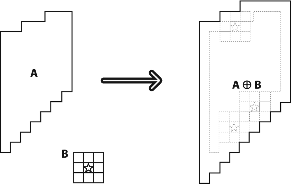
Dilation is a convolution of some image (or region of an image), which we will call A, with some kernel, which we will call B. The kernel, which can be any shape or size, has a single defined anchor point. Most often, the kernel is a small solid square or disk with the anchor point at the center. The kernel can be thought of as a template or mask, and its effect for dilation is that of a local maximum operator. As the kernel B is scanned over the image, we compute the maximal pixel value overlapped by B and replace the image pixel under the anchor point with that maximal value. This causes bright regions within an image to grow as diagrammed in Figure 5-6. This growth is the origin of the term "dilation operator".
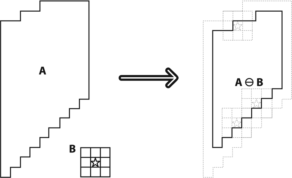
Erosion is the converse operation. The action of the erosion operator is equivalent to computing a local minimum over the area of the kernel. Erosion generates a new image from the original using the following algorithm: as the kernel B is scanned over the image, we compute the minimal pixel value overlapped by B and replace the image pixel under the anchor point with that minimal value.[51] Erosion is diagrammed in Figure 5-7.
Tip
Image morphology is often done on Boolean images that result from thresholding. However, because dilation is just a max operator and erosion is just a min operator, morphology may be used on intensity images as well.
In general, whereas dilation expands region A, erosion reduces region A. Moreover, dilation will tend to smooth concavities and erosion will tend to smooth away protrusions. Of course, the exact result will depend on the kernel, but these statements are generally true so long as the kernel is both convex and filled.
In OpenCV, we effect these transformations using the cvErode() and cvDilate()
functions:
void cvErode(
   IplImage*       src,
   IplImage*       dst,
   IplConvKernel*  B          = NULL,
   int             iterations = 1
);
void cvDilate(
   IplImage*       src,
   IplImage*       dst,
   IplConvKernel*  B          = NULL,
   int             iterations = 1
);
Both cvErode() and cvDilate() take a source and destination image, and both support "in place"
calls (in which the source and destination are the same image). The third argument is the
kernel, which defaults to NULL. In the NULL case, the kernel used is a 3-by-3 kernel with the anchor
at its center (we will discuss shortly how to create your own kernels). Finally, the
fourth argument is the number of iterations. If not set to the default value of 1, the
operation will be applied multiple times during the single call to the function. The
results of an erode operation are shown in Figure 5-8 and those of a dilation operation in Figure 5-9. The erode operation is often used to eliminate "speckle" noise in an image. The idea here is that the speckles are eroded to
nothing while larger regions that contain visually significant content are not affected.
The dilate operation is often used when attempting to find connected components (i.e., large discrete regions of similar pixel color or
intensity). The utility of dilation arises because in many cases a large region might otherwise be broken
apart into multiple components as a result of noise, shadows, or some other similar
effect. A small dilation will cause such components to "melt" together into one.
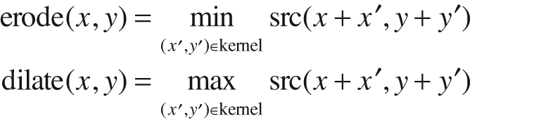
To recap: when OpenCV processes the cvErode()
function, what happens beneath the hood is that the value of some point p is set to the minimum value of all of the points covered by
the kernel when aligned at p; for the dilation
operator, the equation is the same except that max is considered rather than min:
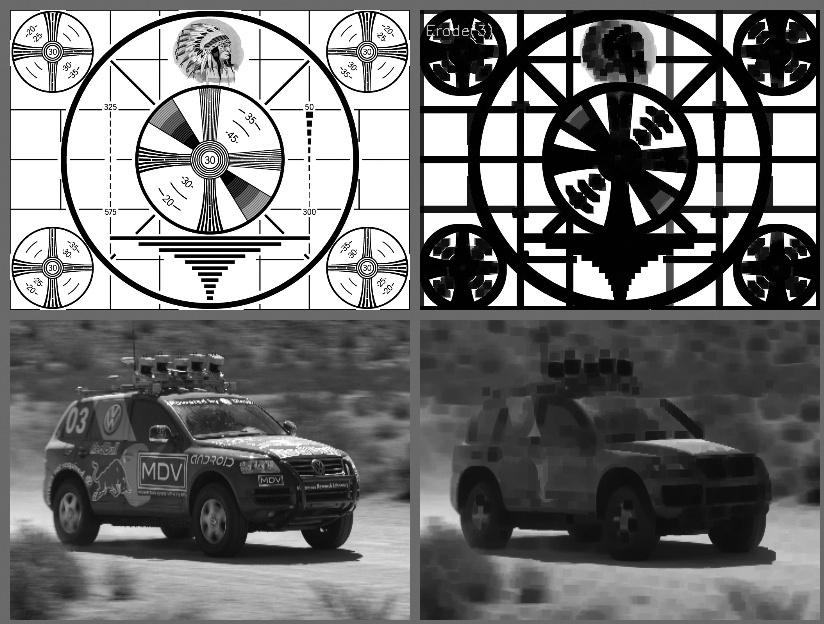
You might be wondering why we need a complicated formula when the earlier heuristic description was perfectly sufficient. Some readers actually prefer such formulas but, more importantly, the formulas capture some generality that isn't apparent in the qualitative description. Observe that if the image is not Boolean then the min and max operators play a less trivial role. Take another look at Figures Figure 5-8 and Figure 5-9, which show the erosion and dilation operators applied to two real images.
You are not limited to the simple 3-by-3 square kernel. You can make your own
custom morphological kernels (our previous "kernel B") using IplConvKernel. Such kernels are allocated using cvCreateStructuringElementEx() and are released using cvReleaseStructuringElement().
IplConvKernel* cvCreateStructuringElementEx(
   int          cols,
   int          rows,
   int          anchor_x,
   int          anchor_y,
   int          shape,
   int*         values=NULL
);

void cvReleaseStructuringElement( IplConvKernel** element );

Figure 5-9. Results of the dilation, or "max", operator: bright regions are expanded and often joined
A morphological kernel, unlike a convolution kernel, doesn't require any
numerical values. The elements of the kernel simply indicate where the max or min
computations take place as the kernel moves around the image. The anchor point indicates
how the kernel is to be aligned with the source image and also where the result of the
computation is to be placed in the destination image. When creating the kernel, cols and rows indicate the
size of the rectangle that holds the structuring element. The next parameters, anchor_x and anchor_y, are
the (x, y) coordinates of the anchor point within the
enclosing rectangle of the kernel. The fifth parameter, shape, can take on values listed in Table 5-2. If CV_SHAPE_CUSTOM is used, then the integer vector values is used to define a custom shape of the kernel within the rows-by-cols enclosing rectangle. This
vector is read in raster scan order with each entry representing a different pixel in the
enclosing rectangle. Any nonzero value is taken to indicate that the corresponding pixel
should be included in the kernel. If values is NULL then the custom shape is interpreted to be all nonzero, resulting in a rectangular
kernel.[52]
When working with Boolean images and image masks, the basic erode and dilate operations are usually sufficient. When
working with grayscale or color images, however, a number of additional operations are
often helpful. Several of the more useful operations can be handled by the multi-purpose
cvMorphologyEx() function.
void cvMorphologyEx(
   const CvArr*   src,
   CvArr*         dst,
   CvArr*         temp,
   IplConvKernel* element,
   int            operation,
   int            iterations  = 1
);
In addition to the arguments src, dst, element, and
iterations, which we used with previous operators,
cvMorphologyEx() has two new parameters. The first is
the temp array, which is required for some of the
operations (see Table 5-3). When required, this
array should be the same size as the source image. The second new argument—the really
interesting one—is operation, which selects the
morphological operation that we will do.
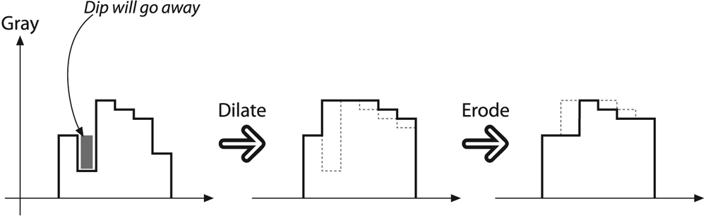
The first two operations in Table 5-3, opening and closing, are combinations of the erosion and dilation operators. In the case of opening, we erode first and then dilate (Figure 5-10). Opening is often used to count regions in a Boolean image. For example, if we have thresholded an image of cells on a microscope slide, we might use opening to separate out cells that are near each other before counting the regions. In the case of closing, we dilate first and then erode (Figure 5-12). Closing is used in most of the more sophisticated connected-component algorithms to reduce unwanted or noise-driven segments. For connected components, usually an erosion or closing operation is performed first to eliminate elements that arise purely from noise and then an opening operation is used to connect nearby large regions. (Notice that, although the end result of using open or close is similar to using erode or dilate, these new operations tend to preserve the area of connected regions more accurately.)
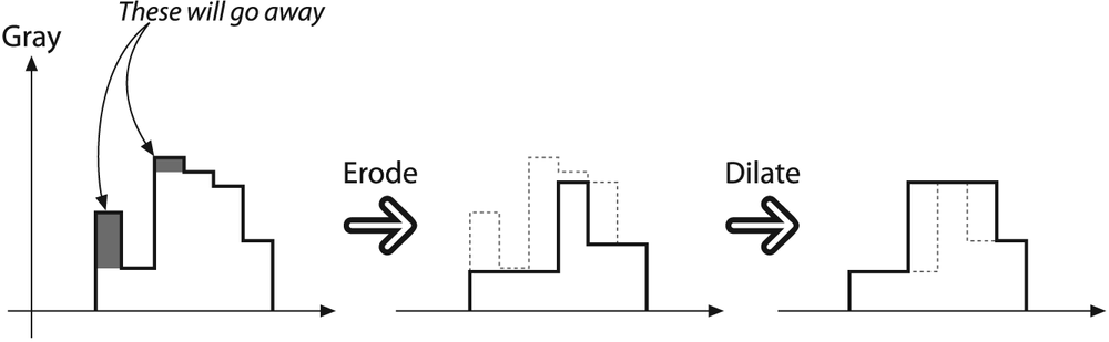
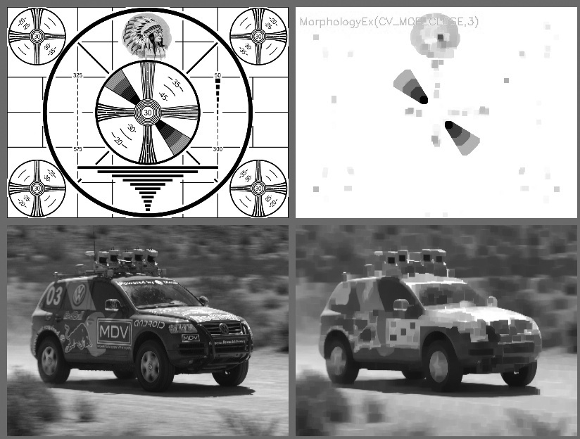
Both the opening and closing operations are approximately area-preserving: the most prominent effect of closing is to eliminate lone outliers that are lower than their neighbors whereas the effect of opening is to eliminate lone outliers that are higher than their neighbors. Results of using the opening operator are shown in Figure 5-11, and of the closing operator in Figure 5-13.
One last note on the opening and closing operators concerns how the iterations argument is interpreted. You might expect that
asking for two iterations of closing would yield something like
dilate-erode-dilate-erode. It turns out that this would not be particularly useful. What
you really want (and what you get) is dilate-dilate-erode-erode. In this way, not only
the single outliers but also neighboring pairs of outliers will disappear.
Our next available operator is the morphological gradient. For this one it is probably easier to start with a formula and then figure out what it means:
| gradient(src) = dilate(src)–erode(src) |
The effect of this operation on a Boolean image would be simply to isolate perimeters of existing blobs. The process is diagrammed in Figure 5-14, and the effect of this operator on our test images is shown in Figure 5-15.
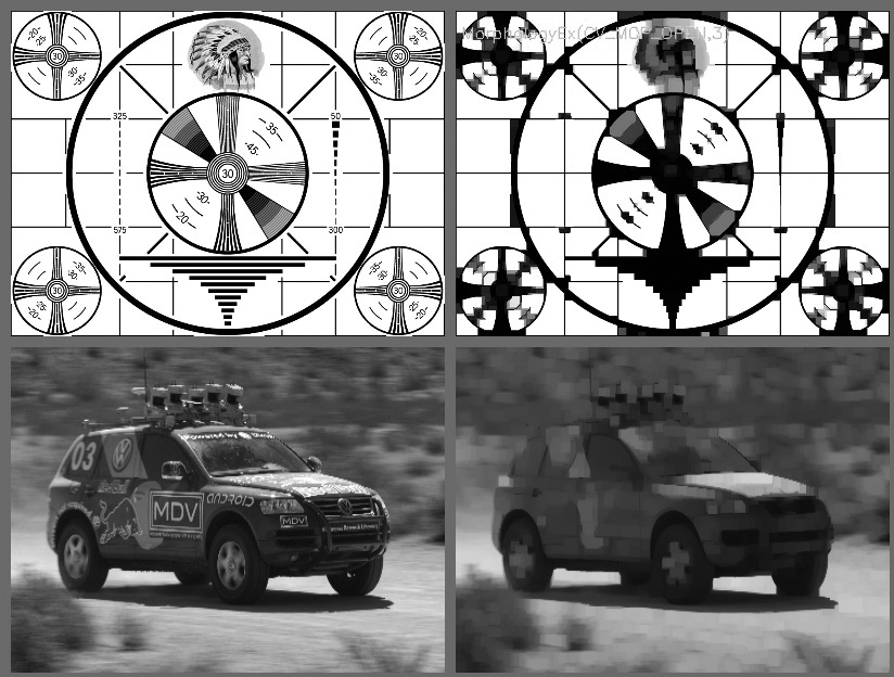
Figure 5-11. Results of morphological opening on an image: small bright regions are removed, and the remaining bright regions are isolated but retain their size
With a grayscale image we see that the value of the operator is telling us something about how fast the image brightness is changing; this is why the name "morphological gradient" is justified. Morphological gradient is often used when we want to isolate the perimeters of bright regions so we can treat them as whole objects (or as whole parts of objects). The complete perimeter of a region tends to be found because an expanded version is subtracted from a contracted version of the region, leaving a complete perimeter edge. This differs from calculating a gradient, which is much less likely to work around the full perimeter of an object.[53]
The last two operators are called Top Hat and Black Hat [Meyer78]. These operators are used to isolate patches that are, respectively, brighter or dimmer than their immediate neighbors. You would use these when trying to isolate parts of an object that exhibit brightness changes relative only to the object to which they are attached. This often occurs with microscope images of organisms or cells, for example. Both operations are defined in terms of the more primitive operators, as follows:
| TopHat(src) = src–open(src) |
| BlackHat(src) = close(src)–src |
As you can see, the Top Hat operator subtracts the opened form of A from A. Recall that the effect of the open operation was to exaggerate small cracks or local drops. Thus, subtracting open(A) from A should reveal areas that are lighter than the surrounding region of A, relative to the size of the kernel (see Figure 5-16); conversely, the Black Hat operator reveals areas that are darker than the surrounding region of A (Figure 5-17). Summary results for all the morphological operators discussed in this chapter are assembled in Figure 5-18.[54]
[51] To be precise, the pixel in the destination image is set to the value equal to the minimal value of the pixels under the kernel in the source image.
[52] If the use of this strange integer vector strikes you as being incongruous with other OpenCV functions, you are not alone. The origin of this syntax is the same as the origin of the IPL prefix to this function—another instance of archeological code relics.
[53] We will return to the topic of gradients when we introduce the Sobel and Scharr operators in the next chapter.
[54] Both of these operations (Top Hat and Black Hat) make more sense in grayscale morphology, where the structuring element is a matrix of real numbers (not just a Boolean mask) and the matrix is added to the current pixel neighborhood before taking a minimum or maximum. Unfortunately, this is not yet implemented in OpenCV.