Image pyramids [Adelson84] are heavily used in a wide variety of vision applications. An image pyramid is a collection of images—all arising from a single original image—that are successively downsampled until some desired stopping point is reached. (Of course, this stopping point could be a single-pixel image!)
There are two kinds of image pyramids that arise often in the literature and in application: the Gaussian [Rosenfeld80] and Laplacian [Burt83] pyramids [Adelson84]. The Gaussian pyramid is used to downsample images, and the Laplacian pyramid (to be discussed shortly) is required when we want to reconstruct an upsampled image from an image lower in the pyramid.
To produce layer (i+1) in the Gaussian pyramid (we denote this layer Gi+1) from layer Gi of the pyramid, we first convolve Gi with a Gaussian kernel and then remove every even-numbered row and column. Of course, from this it follows immediately that each image is exactly one-quarter the area of its predecessor. Iterating this process on the input image G0 produces the entire pyramid. OpenCV provides us with a method for generating each pyramid stage from its predecessor:
void cvPyrDown(
   IplImage*   src,
   IplImage*   dst,
   int         filter = IPL_GAUSSIAN_5x5
);
Currently, the last argument filter supports only the
single (default) option of a 5-by-5 Gaussian kernel.
Similarly, we can convert an existing image to an image that is twice as large in each direction by the following analogous (but not inverse!) operation:
void cvPyrUp(
   IplImage*   src,
   IplImage*   dst,
   int         filter = IPL_GAUSSIAN_5x5
);
In this case the image is first upsized to twice the original in each dimension, with the new (even) rows filled with 0s. Thereafter, a convolution is performed with the given filter (actually, a filter twice as large in each dimension than that specified)[58] to approximate the values of the "missing" pixels.
We noted previously that the operator PyrUp() is not
the inverse of PyrDown(). This should be evident because
PyrDown() is an operator that loses information. In
order to restore the original (higher-resolution) image, we would require access to the
information that was discarded by the downsampling. This data forms the Laplacian pyramid. The ith layer of the
Laplacian pyramid is defined by the relation:
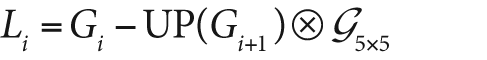
Here the operator UP() upsizes by mapping each pixel
in location (x, y) in the original image to pixel
(2x + 1, 2y + 1) in the destination image; the
 symbol denotes convolution; and
G5x5 is a 5-by-5 Gaussian kernel. Of course,
Gi —
UP(Gi+1)
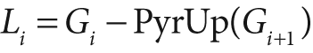
G5x5 is the definition of the
symbol denotes convolution; and
G5x5 is a 5-by-5 Gaussian kernel. Of course,
Gi —
UP(Gi+1)
G5x5 is the definition of the PyrUp() operator provided by OpenCv. Hence, we can use OpenCv to
compute the Laplacian operator directly as:
The Gaussian and Laplacian pyramids are shown diagrammatically in Figure 5-21, which also shows the inverse process for recovering the original image from the subimages. Note how the Laplacian is really an approximation that uses the difference of Gaussians, as revealed in the preceding equation and diagrammed in the figure.

There are many operations that can make extensive use of the Gaussian and Laplacian pyramids, but a particularly important one is image segmentation (see Figure 5-22). In this case, one builds an image pyramid and then associates to it a system of parent–child relations between pixels at level Gi+1 and the corresponding reduced pixel at level Gi. In this way, a fast initial segmentation can be done on the low-resolution images high in the pyramid and then can be refined and further differentiated level by level.
This algorithm (due to B. Jaehne [Jaehne95; Antonisse82]) is implemented in OpenCV as cvPyrSegmentation():
void cvPyrSegmentation(
   IplImage*     src,
   IplImage*     dst,
   CvMemStorage* storage,
   CvSeq**       comp,
   int           level,
   double        threshold1,
   double        threshold2
);

Figure 5-22. Pyramid segmentation with threshold1 set to 150 and threshold2 set to 30; the images on the right contain only a subsection of the images on the left because pyramid segmentation requires images that are N-times divisible by 2, where N is the number of pyramid layers to be computed (these are 512-by-512 areas from the original images)
As usual, src and dst are the source and destination images, which must both be 8-bit, of the
same size, and of the same number of channels (one or three). You might be wondering, "What
destination image?" Not an unreasonable question, actually. The destination image dst is used as scratch space for the algorithm and also as a
return visualization of the segmentation. If you view this image, you will see that each
segment is colored in a single color (the color of some pixel in that segment). Because this
image is the algorithm's scratch space, you cannot simply set it to NULL. Even if you do not want the result, you must provide an image. One
important word of warning about src and dst: because all levels of the image pyramid must have integer
sizes in both dimensions, the starting images must be divisible by two as many times as
there are levels in the pyramid. For example, for a four-level pyramid, a height or width of
80 (2 x 2 x 2 x 5) would be acceptable, but a value of 90 (2 x 3 x 3 x 5) would
not.[59]
The pointer storage is for an OpenCV memory storage
area. In Chapter 8 we will discuss such areas in more detail, but for now
you should know that such a storage area is allocated with a command like[60]
CvMemStorage* storage = cvCreateMemStorage();
The argument comp is a location for storing further
information about the resulting segmentation: a sequence of connected components is
allocated from this memory storage. Exactly how this works will be detailed in Chapter 8, but for convenience here we briefly summarize what you'll need in
the context of cvPyrSegmentation().
First of all, a sequence is essentially a list of structures of a particular kind. Given a sequence, you can obtain the number of elements as well as a particular element if you know both its type and its number in the sequence. Take a look at the Example 5-1 approach to accessing a sequence.
Example 5-1. Doing something with each element in the sequence of connected components returned by cvPyrSegmentation()
void f(

   IplImage* src,
   IplImage* dst
) {
   CvMemStorage* storage = cvCreateMemStorage(0);
   CvSeq* comp = NULL;
   cvPyrSegmentation( src, dst, storage, &comp, 4, 200, 50 );
   int n_comp = comp->total;
   for( int i=0; i<n_comp; i++ ) {
     CvConnectedComp* cc = (CvConnectedComp*) cvGetSeqElem( comp, i );
     do_something_with( cc );
   }
   cvReleaseMemStorage( &storage );
}
There are several things you should notice in this example. First, observe the
allocation of a memory storage; this is where cvPyrSegmentation() will get the memory it needs for the
connected components it will have to create. Then the pointer comp is allocated as type CvSeq*. It is
initialized to NULL because its current value means
nothing. We will pass to cvPyrSegmentation() a pointer to
comp so that comp
can be set to the location of the sequence created by cvPyrSegmentation(). Once we have called the segmentation, we can figure out
how many elements there are in the sequence with the member element total. Thereafter we can use the generic cvGetSeqElem() to obtain the ith element of comp; however, because cvGetSeqElem() is
generic and returns only a void pointer, we must cast the return pointer to the appropriate
type (in this case, CvConnectedComp*).
Finally, we need to know that a connected component is one of the basic structure types in OpenCV. You can think of it as a way of describing a "blob" in an image. It has the following definition:
typedef struct CvConnectedComponent {
  double area;
  CvScalar value;
  CvRect rect;
  CvSeq* contour;
};
The area is the area of the component. The value is the average color[61] over the area of the component and rect is a
bounding box for the component (defined in the coordinates of the parent image). The final element, contour, is a pointer to another sequence. This sequence can be
used to store a representation of the boundary of the component, typically as a sequence of
points (type CvPoint).
In the specific case of cvPyrSegmentation(), the
contour member is not set. Thus, if you want some specific representation of the component's
pixels then you will have to compute it yourself. The method to use depends, of course, on
the representation you have in mind. Often you will want a Boolean mask with nonzero elements wherever the component was located. You can
easily generate this by using the rect portion of the
connected component as a mask and then using cvFloodFill() to select the desired pixels inside of that rectangle.
[58] This filter is also normalized to four, rather than to one. This is appropriate because the inserted rows have 0s in all of their pixels before the convolution.
[59] Heed this warning! Otherwise, you will get a totally useless error message and probably waste hours trying to figure out what's going on.
[60] Actually, the current implementation of cvPyrSegmentation() is a bit incomplete in that it returns not the computed
segments but only the bounding rectangles (as CvSeq<CvConnectedComp>).
[61] Actually the meaning of value is context
dependant and could be just about anything, but it is typically a color associated with
the component. In the case of cvPyrSegmentation(),
value is the average color over the segment.