The Hough transform[68] is a method for finding lines, circles, or other simple forms in an image. The original Hough transform was a line transform, which is a relatively fast way of searching a binary image for straight lines. The transform can be further generalized to cases other than just simple lines.
The basic theory of the Hough line transform is that any point in a binary image could be part of some set of possible lines. If we parameterize each line by, for example, a slope a and an intercept b, then a point in the original image is transformed to a locus of points in the (a, b) plane corresponding to all of the lines passing through that point (see Figure 6-9). If we convert every nonzero pixel in the input image into such a set of points in the output image and sum over all such contributions, then lines that appear in the input (i.e., (x, y) plane) image will appear as local maxima in the output (i.e., (a, b) plane) image. Because we are summing the contributions from each point, the (a, b) plane is commonly called the accumulator plane.

Figure 6-8. Results of Canny edge detection for two different images when the high and low thresholds are set to 150 and 100, respectively
It might occur to you that the slope-intercept form is not really the best way to represent all of the lines passing through a point (because of the considerably different density of lines as a function of the slope, and the related fact that the interval of possible slopes goes from –∞ to +∞). It is for this reason that the actual parameterization of the transform image used in numerical computation is somewhat different. The preferred parameterization represents each line as a point in polar coordinates (ρ, θ), with the implied line being the line passing through the indicated point but perpendicular to the radial from the origin to that point (see Figure 6-10). The equation for such a line is:

Figure 6-9. The Hough line transform finds many lines in each image; some of the lines found are expected, but others may not be

Figure 6-10. A point (x0, y0) in the image plane (panel a) implies many lines each parameterized by a different ρ and θ (panel b); these lines each imply points in the (ρ, θ) plane, which taken together form a curve of characteristic shape (panel c)
The OpenCV Hough transform algorithm does not make this computation explicit to the user. Instead, it simply returns the local maxima in the (ρ, θ) plane. However, you will need to understand this process in order to understand the arguments to the OpenCV Hough line transform function.
OpenCV supports two different kinds of Hough line transform: the standard Hough transform (SHT) [Duda72] and the progressive probabilistic Hough transform (PPHT). [69] The SHT is the algorithm we just looked at. The PPHT is a variation of this algorithm that, among other things, computes an extent for individual lines in addition to the orientation (as shown in Figure 6-11). It is "probabilistic" because, rather than accumulating every possible point in the accumulator plane, it accumulates only a fraction of them. The idea is that if the peak is going to be high enough anyhow, then hitting it only a fraction of the time will be enough to find it; the result of this conjecture can be a substantial reduction in computation time. Both of these algorithms are accessed with the same OpenCV function, though the meanings of some of the arguments depend on which method is being used.
CvSeq* cvHoughLines2(
  CvArr* image,
  void*  line_storage,
  int    method,
  double rho,
  double theta,
  int    threshold,
  double param1      = 0,
  double param2      = 0
);
The first argument is the input image. It must be an 8-bit image, but the input is
treated as binary information (i.e., all nonzero pixels are considered to be equivalent).
The second argument is a pointer to a place where the results can be stored, which can be
either a memory storage (see CvMemoryStorage in Chapter 8) or a plain N-by-1 matrix array (the number of
rows, N, will serve to limit the maximum number of lines returned).
The next argument, method, can be CV_HOUGH_STANDARD, CV_HOUGH_PROBABILISTIC, or CV_HOUGH_MULTI_SCALE for (respectively) SHT, PPHT, or a
multiscale variant of SHT.
The next two arguments, rho and theta, set the resolution desired for the lines (i.e., the
resolution of the accumulator plane). The units of rho
are pixels and the units of theta are radians; thus,
the accumulator plane can be thought of as a two-dimensional histogram with cells of
dimension rho pixels by theta radians. The threshold value is the
value in the accumulator plane that must be reached for the routine to report a line. This
last argument is a bit tricky in practice; it is not normalized, so you should expect to
scale it up with the image size for SHT. Remember that this argument is, in effect,
indicating the number of points (in the edge image) that must support the line for the
line to be returned.

Figure 6-11. The Canny edge detector (param1=50, param2=150) is run first, with the results shown in gray, and the progressive probabilistic Hough transform (param1=50, param2=10) is run next, with the results overlayed in white; you can see that the strong lines are generally picked up by the Hough transform
The param1 and param2 arguments are not used by the SHT. For the PPHT, param1 sets the minimum length of a line segment that will be
returned, and param2 sets the separation between
collinear segments required for the algorithm not to join them into a single longer
segment. For the multiscale HT, the two parameters are used to indicate higher resolutions
to which the parameters for the lines should be computed. The multiscale HT first computes
the locations of the lines to the accuracy given by the rho and theta parameters and then goes on
to refine those results by a factor of param1 and
param2, respectively (i.e., the final resolution in
rho is rho divided
by param1 and the final resolution in theta is theta divided by
param2).
What the function returns depends on how it was called. If the line_storage value was a matrix array, then the actual return
value will be NULL. In this case, the matrix should be
of type CV_32FC2 if the SHT or multi-scale HT is being
used and should be CV_32SC4 if the PPHT is being used.
In the first two cases, the ρ- and θ-values for
each line will be placed in the two channels of the array. In the case of the PPHT, the
four channels will hold the x- and y-values of
the start and endpoints of the returned segments. In all of these cases, the number of
rows in the array will be updated by cvHoughLines2() to
correctly reflect the number of lines returned.
If the line_storage value was a pointer to a memory
store, [70] then the return value will be a pointer to a CvSeq sequence structure. In that case, you can get each line or line segment
from the sequence with a command like
float* line = (float*) cvGetSeqElem( lines , i );
where lines is the return value from cvHoughLines2() and i is
index of the line of interest. In this case, line will
be a pointer to the data for that line, with line[0]
and line[1] being the floating-point values
ρ and θ (for SHT and MSHT) or CvPoint structures for the endpoints of the segments (for
PPHT).
The Hough circle transform [Kimme75] (see Figure 6-12) works in a manner roughly analogous to the Hough line transforms just described. The reason it is only "roughly" is that—if one were to try doing the exactly analogous thing—the accumulator plane would have to be replaced with an accumulator volume with three dimensions: one for x, one for y, and another for the circle radius r. This would mean far greater memory requirements and much slower speed. The implementation of the circle transform in OpenCV avoids this problem by using a somewhat more tricky method called the Hough gradient method.
The Hough gradient method works as follows. First the image is passed through an edge
detection phase (in this case, cvCanny()). Next, for
every nonzero point in the edge image, the local gradient is considered (the gradient is
computed by first computing the first-order Sobel x- and y-derivatives via
cvSobel()). Using this gradient, every point along
the line indicated by this slope—from a specified minimum to a specified maximum
distance—is incremented in the accumulator. At the same time, the location of every one of
these nonzero pixels in the edge image is noted. The candidate centers are then selected
from those points in this (two-dimensional) accumulator that are both above some given
threshold and larger than all of their immediate neighbors. These candidate centers are
sorted in descending order of their accumulator values, so that the centers with the most
supporting pixels appear first. Next, for each center, all of the nonzero pixels (recall
that this list was built earlier) are considered. These pixels are sorted according to
their distance from the center. Working out from the smallest distances to the maximum
radius, a single radius is selected that is best supported by the nonzero pixels. A center
is kept if it has sufficient support from the nonzero pixels in the edge image
and if it is a sufficient distance from any previously selected
center.
This implementation enables the algorithm to run much faster and, perhaps more importantly, helps overcome the problem of the otherwise sparse population of a three-dimensional accumulator, which would lead to a lot of noise and render the results unstable. On the other hand, this algorithm has several shortcomings that you should be aware of.
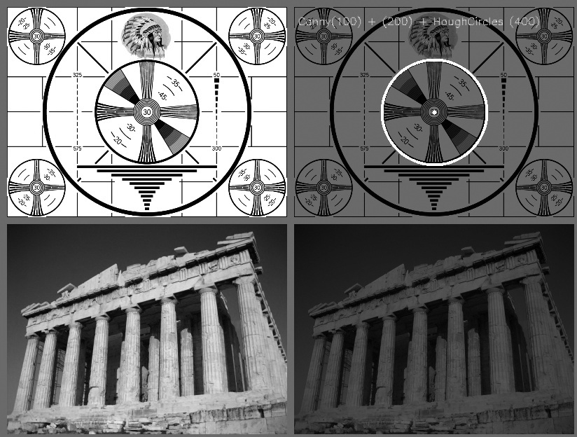
Figure 6-12. The Hough circle transform finds some of the circles in the test pattern and (correctly) finds none in the photograph
First, the use of the Sobel derivatives to compute the local gradient—and the attendant assumption that this can be considered equivalent to a local tangent—is not a numerically stable proposition. It might be true "most of the time," but you should expect this to generate some noise in the output.
Second, the entire set of nonzero pixels in the edge image is considered for every candidate center; hence, if you make the accumulator threshold too low, the algorithm will take a long time to run. Third, because only one circle is selected for every center, if there are concentric circles then you will get only one of them.
Finally, because centers are considered in ascending order of their associated accumulator value and because new centers are not kept if they are too close to previously accepted centers, there is a bias toward keeping the larger circles when multiple circles are concentric or approximately concentric. (It is only a "bias" because of the noise arising from the Sobel derivatives; in a smooth image at infinite resolution, it would be a certainty.)
With all of that in mind, let's move on to the OpenCV routine that does all this for us:
CvSeq* cv HoughCircles(
  CvArr* image,
  void*  circle_storage,
  int    method,
  double dp,
  double min_dist,
  double param1     = 100,
  double param2     = 300,
  int    min_radius = 0,
  int    max_radius = 0
);
The Hough circle transform function cvHoughCircles()
has similar arguments to the line transform. The input image is again an 8-bit image. One significant difference between cvHoughCircles() and cvHoughLines2() is that the latter requires a binary image. The cvHoughCircles() function will internally (automatically) call
cvSobel()
[71] for you, so you can provide a more general grayscale image.
The circle_storage can be either an array or memory
storage, depending on how you would like the results returned. If an array is used, it
should be a single column of type CV_32FC3; the three
channels will be used to encode the location of the circle and its radius. If memory
storage is used, then the circles will be made into an OpenCV sequence and a pointer to
that sequence will be returned by cvHoughCircles().
(Given an array pointer value for circle_storage, the
return value of cvHoughCircles() is NULL.) The method argument
must always be set to CV_HOUGH_GRADIENT.
The parameter dp is the resolution of the
accumulator image used. This parameter allows us to create an accumulator of a lower
resolution than the input image. (It makes sense to do this because there is no reason to
expect the circles that exist in the image to fall naturally into the same number of bins
as the width or height of the image itself.) If dp is
set to 1 then the resolutions will be the same; if set to a larger number (e.g., 2), then
the accumulator resolution will be smaller by that factor (in this case, half). The value
of dp cannot be less than 1.
The parameter min_dist is the minimum distance that
must exist between two circles in order for the algorithm to consider them distinct
circles.
For the (currently required) case of the method being set to CV_HOUGH_GRADIENT, the next two arguments, param1 and param2, are the edge (Canny)
threshold and the accumulator threshold, respectively. You may recall that the Canny edge detector actually takes two different thresholds itself. When
cvCanny() is called internally, the first (higher)
threshold is set to the value of param1 passed into
cvHoughCircles(), and the second (lower) threshold is
set to exactly half that value. The parameter param2 is
the one used to threshold the accumulator and is exactly analogous to the threshold argument of cvHoughLines().
The final two parameters are the minimum and maximum radius of circles that can be
found. This means that these are the radii of circles for which the accumulator has a
representation. Example 6-1 shows an
example program using cvHoughCircles().
Example 6-1. Using cvHoughCircles to return a sequence of circles found in a grayscale image
#include <cv.h>
#include <highgui.h>
#include <math.h>

int main(int argc, char** argv) {
  IplImage* image = cvLoadImage(
    argv[1],
    CV_LOAD_IMAGE_GRAYSCALE
  );

  CvMemStorage* storage = cvCreateMemStorage(0);
  cvSmooth(image, image, CV_GAUSSIAN, 5, 5 );

  CvSeq* results = cvHoughCircles(
    image,
    storage,
    CV_HOUGH_GRADIENT,
    2,
    image->width/10
  );

  for( int i = 0; i < results->total; i++ ) {
    float* p = (float*) cvGetSeqElem( results, i );
    CvPoint pt = cvPoint( cvRound( p[0] ), cvRound( p[1] ) );
    cvCircle(
      image,
      pt,
      cvRound( p[2] ),
      CV_RGB(0xff,0xff,0xff)
   );
  }
  cvNamedWindow( "cvHoughCircles", 1 );
  cvShowImage( "cvHoughCircles", image);
  cvWaitKey(0);
}
It is worth reflecting momentarily on the fact that, no matter what tricks we employ, there is no getting around the requirement that circles be described by three degrees of freedom (x, y, and r), in contrast to only two degrees of freedom (ρ and θ) for lines. The result will invariably be that any circle-finding algorithm requires more memory and computation time than the line-finding algorithms we looked at previously. With this in mind, it's a good idea to bound the radius parameter as tightly as circumstances allow in order to keep these costs under control. [72] The Hough transform was extended to arbitrary shapes by Ballard in 1981 [Ballard81] basically by considering objects as collections of gradient edges.
[68] Hough developed the transform for use in physics experiments [Hough59]; its use in vision was introduced by Duda and Hart [Duda72].
[69] The "probablistic Hough transform" (PHT) was introduced by Kiryati, Eldar, and Bruckshtein in 1991 [Kiryati91]; the PPHT was introduced by Matas, Galambosy, and Kittler in 1999 [Matas00].
[70] We have not yet introduced the concept of a memory store or a sequence, but Chapter 8 is devoted to this topic.
[71] The function cvSobel(), not cvCanny(), is called internally. The reason is that
cvHoughCircles() needs to estimate the
orientation of a gradient at each pixel, and this is difficult to do with binary edge
map.
[72] Although cvHoughCircles() catches centers of
the circles quite well, it sometimes fails to find the correct radius. Therefore, in
an application where only a center must be found (or where some different technique
can be used to find the actual radius), the radius returned by cvHoughCircles() can be ignored.