LogPolar

For two-dimensional images, the log-polar transform [Schwartz80] is a change from Cartesian to polar coordinates:

, where

and

. Next, to separate out the polar coordinates into a (ρ, θ) space that is relative to some center point (x_c, y_c), we take the log so that

and

. For image purposes—when we need to "fit" the interesting stuff into the available image memory—we typically apply a scaling factor m to ρ. Figure 6-15 shows a square object on the left and its encoding in log-polar space.

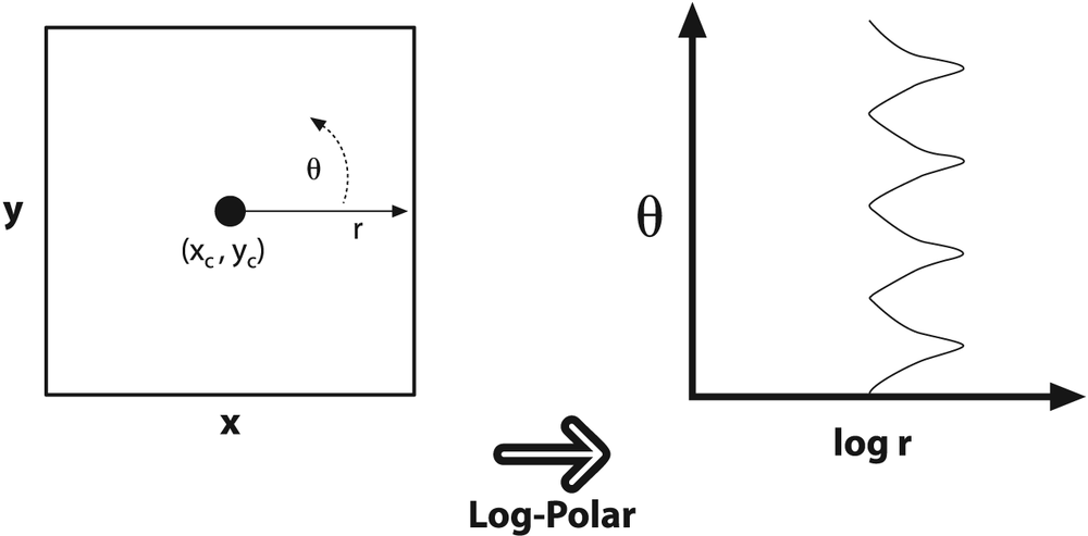
Figure 6-15. The log-polar transform maps (x, y) into (log(r),θ); here, a square is displayed in the log-polar coordinate system

The next question is, of course, "Why bother?" The log-polar transform takes its inspiration from the human visual system. Your eye has a small but dense center of photoreceptors in its center (the fovea), and the density of receptors fall off rapidly (exponentially) from there. Try staring at a spot on the wall and holding your finger at arm's length in your line of sight. Then, keep staring at the spot and move your finger slowly away; note how the detail rapidly decreases as the image of your finger moves away from your fovea. This structure also has certain nice mathematical properties (beyond the scope of this book) that concern preserving the angles of line intersections.

More important for us is that the log-polar transform can be used to create two-dimensional invariant representations of object views by shifting the transformed image's center of mass to a fixed point in the log-polar plane; see Figure 6-16. On the left are three shapes that we want to recognize as "square". The problem is, they look very different. One is much larger than the others and another is rotated. The log-polar transform appears on the right in Figure 6-16. Observe that size differences in the (x, y) plane are converted to shifts along the log(r) axis of the log-polar plane and that the rotation differences are converted to shifts along the θ-axis in the log-polar plane. If we take the transformed center of each transformed square in the log-polar plane and then recenter that point to a certain fixed position, then all the squares will show up identically in the log-polar plane. This yields a type of invariance to two-dimensional rotation and scaling. ^[80]

Figure 6-16. Log-polar transform of rotated and scaled squares: size goes to a shift on the log(r) axis and rotation to a shift on the θ-axis

The OpenCV function for a log-polar transform is cvLogPolar():

void cvLogPolar(
  const CvArr* src,
  CvArr*       dst,
  CvPoint2D32f center,
  double       m,
  int          flags = CV_INTER_LINEAR | CV_WARP_FILL_OUTLIERS
);

The src and dst are one- or three-channel color or grayscale images. The parameter center is the center point (x_c, y_c) of the log-polar transform; m is the scale factor, which should be set so that the features of interest dominate the available image area. The flags parameter allows for different interpolation methods. The interpolation methods are the same set of standard interpolations available in OpenCV (Table 6-1). The interpolation methods can be combined with either or both of the flags CV_WARP_FILL_OUTLIERS (to fill points that would otherwise be undefined) or CV_WARP_INVERSE_MAP (to compute the reverse mapping from log-polar to Cartesian coordinates).

Sample log-polar coding is given in Example 6-4, which demonstrates the forward and backward (inverse) log-polar transform. The results on a photographic image are shown in Figure 6-17.

Figure 6-17. Log-polar example on an elk with transform centered at the white circle on the left; the output is on the right

Example 6-4. Log-polar transform example

// logPolar.cpp : Defines the entry point for the console application.
//
#include <cv.h>
#include <highgui.h>

int main(int argc, char** argv) {
  IplImage* src;
  double M;
  if( argc == 3 && ((src=cvLoadImage(argv[1],1)) != 0 )) {
    M = atof(argv[2]);
    IplImage* dst = cvCreateImage( cvGetSize(src), 8, 3 );
    IplImage* src2 = cvCreateImage( cvGetSize(src), 8, 3 );
    cvLogPolar(
      src, 
      dst,
      cvPoint2D32f(src->width/4,src->height/2), 
      M,
      CV_INTER_LINEAR+CV_WARP_FILL_OUTLIERS
      );
      cvLogPolar(
        dst, 
        src2,
        cvPoint2D32f(src->width/4, src->height/2),
        M,
        CV_INTER_LINEAR | CV_WARP_INVERSE_MAP
      );
      cvNamedWindow( "log-polar", 1 );
      cvShowImage( "log-polar", dst );
      cvNamedWindow( "inverse log-polar", 1 );
      cvShowImage( "inverse log-polar", src2 );
      cvWaitKey();
   }
   return 0;
  }

---

^[80] In Chapter 13 we'll learn about recognition. For now simply note that it wouldn't be a good idea to derive a log-polar transform for a whole object because such transforms are quite sensitive to the exact location of their center points. What is more likely to work for object recognition is to detect a collection of key points (such as corners or blob locations) around an object, truncate the extent of such views, and then use the centers of those key points as log-polar centers. These local log-polar transforms could then be used to create local features that are (partially) scale- and rotation-invariant and that can be associated with a visual object.