For any set of values that are indexed by a discrete (integer) parameter, it is possible to define a discrete Fourier transform (DFT)[81] in a manner analogous to the Fourier transform of a continuous function. For N complex numbers
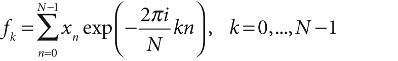
, the one-dimensional DFT is defined by the following formula (where
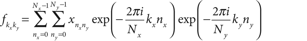
A similar transform can be defined for a two-dimensional array of numbers (of course higher-dimensional analogues exist also):
In general, one might expect that the computation of the N
different terms fk would require
O(N2) operations. In
fact, there are a number of fast Fourier transform (FFT) algorithms
capable of computing these values in O(N log
N) time. The OpenCV function cvDFT() implements one such FFT algorithm. The function cvDFT() can compute FFTs for one- and two-dimensional arrays of
inputs. In the latter case, the two-dimensional transform can be computed or, if desired,
only the one-dimensional transforms of each individual row can be computed (this operation
is much faster than calling cvDFT() many separate
times).
void cvDFT(
  const CvArr* src,
  CvArr*       dst,
  int          flags,
  int          nonzero_rows = 0
);
The input and the output arrays must be floating-point types and may be single- or
double-channel arrays. In the single-channel case, the entries are assumed to be real
numbers and the output will be packed in a special space-saving format (inherited from the
same older IPL library as the IplImage structure). If the
source and channel are two-channel matrices or images, then the two channels will be
interpreted as the real and imaginary components of the input data. In this case, there will
be no special packing of the results, and some space will be wasted with a lot of 0s in both
the input and output arrays. [82]
The special packing of result values that is used with single-channel output is as follows.
For a one-dimensional array:

For a two-dimensional array:
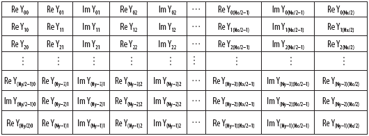
It is worth taking a moment to look closely at the indices on these arrays. The issue here is that certain values are guaranteed to be 0 (more accurately, certain values of fk are guaranteed to be real). It should also be noted that the last row listed in the table will be present only if Ny is even and that the last column will be present only if Nx is even. (In the case of the 2D array being treated as Ny 1D arrays rather than a full 2D transform, all of the result rows will be analogous to the single row listed for the output of the 1D array).
The third argument, called flags, indicates exactly
what operation is to be done. The transformation we started with is known as a
forward transform and is selected with the flag CV_DXT_FORWARD. The inverse transform[83] is defined in exactly the same way except for a change of sign in the
exponential and a scale factor. To perform the inverse transform without the scale factor,
use the flag CV_DXT_INVERSE. The flag for the scale
factor is CV_DXT_SCALE, and this results in all of the
output being scaled by a factor of 1/N (or
1/Nx Ny for a 2D
transform). This scaling is necessary if the sequential application of the forward transform
and the inverse transform is to bring us back to where we started. Because one often wants
to combine CV_DXT_INVERSE with CV_DXT_SCALE, there are several shorthand notations for this kind of operation.
In addition to just combining the two operations with OR, you can use CV_DXT_INV_SCALE (or CV_DXT_INVERSE_SCALE if you're not into that brevity thing). The last flag you
may want to have handy is CV_DXT_ROWS, which allows you
to tell cvDFT() to treat a two-dimensional array as a
collection of one-dimensional arrays that should each be transformed separately as if they
were Ny distinct vectors of length
Nx. This significantly reduces overhead when
doing many transformations at a time (especially when using Intel's optimized IPP libraries). By using CV_DXT_ROWS it is
also possible to implement three-dimensional (and higher) DFT.
In order to understand the last argument, nonzero_rows, we must digress for a moment to explain that in general, DFT
algorithms will strongly prefer vectors of some lengths over other lengths, or arrays of
some sizes over other sizes. In most DFT algorithms, the preferred sizes are powers of 2
(i.e., 2
n
for some integer n). In the case of the algorithm used by OpenCV, the
preference is that the vector lengths, or array dimensions, be 2
p
3
q
5
r
, for some integers p, q, and
r. Hence the usual procedure is to create a somewhat larger array and
then use cvGetSubRect() to copy your array into the
somewhat roomier zero-padded array. For convenience, there is a handy utility function,
cvGetOptimalDFTSize(), which takes the (integer) length of your vector
and returns the first equal or larger size which can be expressed in the form given (i.e.
2p3q5r).
In many applications that involve computing DFTs, one must also compute the
per-element multiplication of two spectra. Because such results are typically packed in
their special high-density format and are usually complex numbers, it would be tedious to
unpack them and handle the multiplication via the "usual" matrix operations. Fortunately,
OpenCV provides the handy cvMulSpectrums() routine,
which performs exactly this function as well as a few other handy things.
void cvMulSpectrums(
   const CvArr* src1,
   const CvArr* src2,
   CvArr*       dst,
   int          flags
);
Note that the first two arguments are the usual input arrays, though in this case they
are spectra from calls to cvDFT(). The third argument
must be a pointer to an array—of the same type and size as the first two—that will be used
for the results. The final argument, flags, tells
cvMulSpectrums() exactly what you want done. In
particular, it may be set to 0 (CV_DXT_FORWARD) for
implementing the above pair multiplication or set to CV_DXT_MUL_CONJ if the element from the first array is to be multiplied by
the complex conjugate of the corresponding element of the second array. The flags may also
be combined with CV_DXT_ROWS in the two-dimensional
case if each array row 0 is to be treated as a separate spectrum (remember, if you created
the spectrum arrays with CV_DXT_ROWS then the data
packing is slightly different than if you created them without that function, so you must
be consistent in the way you call cvMulSpectrums).
It is possible to greatly increase the speed of a convolution by using DFT via the
convolution theorem [Titchmarsh26] that relates convolution in the spatial
domain to multiplication in the Fourier domain [Morse53; Bracewell65; Arfken85]. [84] To accomplish this, one first computes the Fourier transform of the image and
then the Fourier transform of the convolution filter. Once this is done, the convolution
can be performed in the transform space in linear time with respect to the number of
pixels in the image. It is worthwhile to look at the source code for computing such a
convolution, as it also will provide us with many good examples of using cvDFT(). The code is shown in Example 6-5, which is taken directly from the
OpenCV reference.
Example 6-5. Use of cvDFT() to accelerate the computation of convolutions
// Use DFT to accelerate the convolution of array A by kernel B.
// Place the result in array V.
//
void speedy_conv olution(
  const CvMat* A, // Size: M1xN1
  const CvMat* B,  // Size: M2xN2
  CvMat*       C   // Size:(A->rows+B->rows-1)x(A->cols+B->cols-1)
) {

  int dft_M = cvGetOptimalDFTSize( A->rows+B->rows-1 );
  int dft_N = cvGetOptimalDFTSize( A->cols+B->cols-1 );

  CvMat* dft_A = cvCreateMat( dft_M, dft_N, A->type );
  CvMat* dft_B = cvCreateMat( dft_M, dft_N, B->type );
  CvMat tmp;

  // copy A to dft_A and pad dft_A with zeros
  //
  cvGetSubRect( dft_A, &tmp, cvRect(0,0,A->cols,A->rows));
  cvCopy( A, &tmp );
  cvGetSubRect(
    dft_A,
    &tmp,
    cvRect( A->cols, 0, dft_A->cols-A->cols, A->rows )
  );
  cvZero( &tmp );

  // no need to pad bottom part of dft_A with zeros because of
  // use nonzero_rows parameter in cvDFT() call below
  //
  cvDFT( dft_A, dft_A, CV_DXT_FORWARD, A->rows );

  // repeat the same with the second array
  //
  cvGetSubRect( dft_B, &tmp, cvRect(0,0,B->cols,B->rows) );
  cvCopy( B, &tmp );
  cvGetSubRect(
    dft_B,
    &tmp,
    cvRect( B->cols, 0, dft_B->cols-B->cols, B->rows )
  );
  cvZero( &tmp );

  // no need to pad bottom part of dft_B with zeros because of
  // use nonzero_rows parameter in cvDFT() call below
  //
  cvDFT( dft_B, dft_B, CV_DXT_FORWARD, B->rows );

  // or CV_DXT_MUL_CONJ to get correlation rather than convolution
  //
  cvMulSpectrums( dft_A, dft_B, dft_A, 0 );

  // calculate only the top part
  //
  cvDFT( dft_A, dft_A, CV_DXT_INV_SCALE, C->rows );
  cvGetSubRect( dft_A, &tmp, cvRect(0,0,conv->cols,C->rows) );

  cvCopy( &tmp, C );

  cvReleaseMat( dft_A );
  cvReleaseMat( dft_B );
}
In Example 6-5 we can see that the input arrays are first created and then initialized. Next, two new arrays are created whose dimensions are optimal for the DFT algorithm. The original arrays are copied into these new arrays and then the transforms are computed. Finally, the spectra are multiplied together and the inverse transform is applied to the product. The transforms are the slowest[85] part of this operation; an N-by-N image takes O(N2 log N) time and so the entire process is also completed in that time (assuming that N > M for an M-by-M convolution kernel). This time is much faster than O(N2M2), the non-DFT convolution time required by the more naïve method.
[81] Joseph Fourier [Fourier] was the first to find that some functions can be decomposed into an infinite series of other functions, and doing so became a field known as Fourier analysis. Some key text on methods of decomposing functions into their Fourier series are Morse for physics [Morse53] and Papoulis in general [Papoulis62]. The fast Fourier transform was invented by Cooley and Tukeye in 1965 [Cooley65] though Carl Gauss worked out the key steps as early as 1805 [Johnson84]. Early use in computer vision is described by Ballard and Brown [Ballard82].
[82] When using this method, you must be sure to explicitly set the imaginary components
to 0 in the twochannel representation. An easy way to do this is to create a matrix full
of 0s using cvZero() for the imaginary part and then
to call cvMerge() with a real-valued matrix to form a
temporary complex array on which to run cvDFT()
(possibly in-place). This procedure will result in full-size, unpacked, complex matrix
of the spectrum.
[83] With the inverse transform, the input is packed in the special format described
previously. This makes sense because, if we first called the forward DFT and then ran
the inverse DFT on the results, we would expect to wind up with the original data—that
is, of course, if we remember to use the CV_DXT_SCALE
flag!
[84] Recall that OpenCV's DFT algorithm implements the FFT whenever the data size makes the FFT faster.
[85] By "slowest" we mean "asymptotically slowest"—in other words, that this portion of the algorithm takes the most time for very large N. This is an important distinction. In practice, as we saw in the earlier section on convolutions, it is not always optimal to pay the overhead for conversion to Fourier space. In general, when convolving with a small kernel it will not be worth the trouble to make this transformation.