OpenCV allows you to calculate an integral image easily with the appropriately named
cvIntegral() function. An integral
image [Viola04] is a data structure that allows rapid summing of subregions.
Such summations are useful in many applications; a notable one is the computation of
Haar wavelets, which are used in some face recognition and similar
algorithms.
void cvIntegral(
   const CvArr* image,
   CvArr*       sum,
   CvArr*       sqsum      = NULL,
   CvArr*       tilted_sum = NULL
);
The arguments to cvIntegral() are the original image
as well as pointers to destination images for the results. The argument sum is required; the others, sqsum and tilted_sum, may be provided if
desired. (Actually, the arguments need not be images; they could be matrices, but in
practice, they are usually images.) When the input image is 8-bit unsigned, the sum or tilted_sum may be
32-bit integer or floating-point arrays. For all other cases, the sum or tilted_sum must be floating-point
valued (either 32- or 64-bit). The result "images" must always be floating-point. If the
input image is of size W-by-H, then the output
images must be of size (W + 1)-by-(H + 1).
[86]
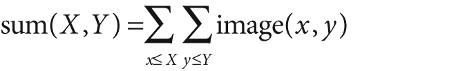
An integral image sum has the form:
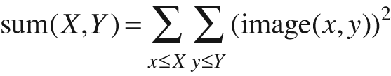
The optional sqsum image is the sum of
squares:
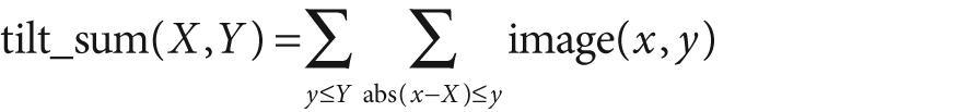
and the tilted_sum is like the sum except that it is
for the image rotated by 45 degrees:
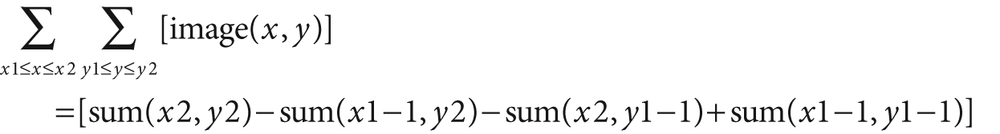
Using these integral images, one may calculate sums, means, and standard deviations over arbitrary upright or "tilted" rectangular regions of the image. As a simple example, to sum over a simple rectangular region described by the corner points (x1, y1) and (x2, y2), where x2 > x1 and y2 > y1, we'd compute:
In this way, it is possible to do fast blurring, approximate gradients, compute means and standard deviations, and perform fast block correlations even for variable window sizes.
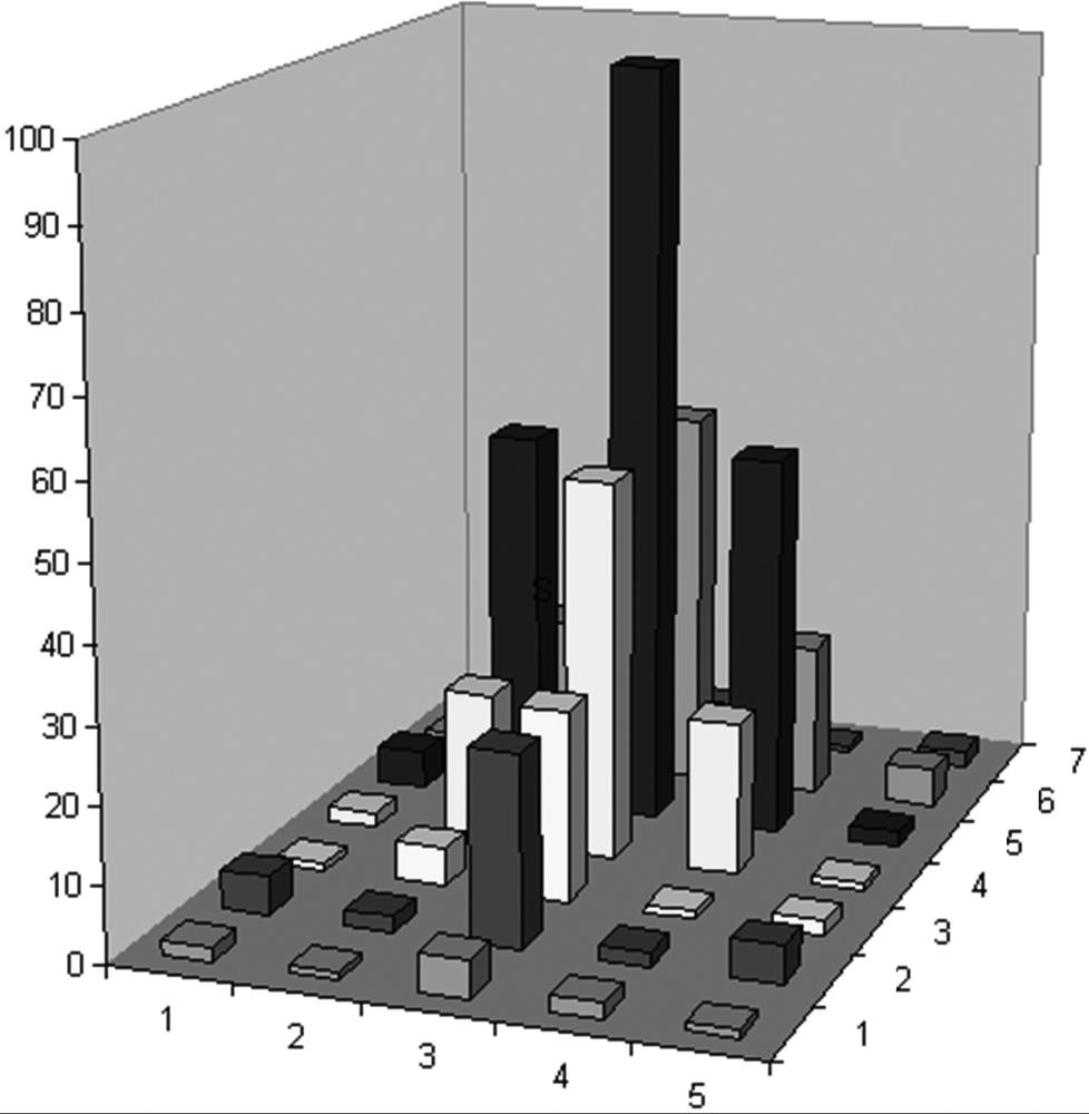
To make this all a little more clear, consider the 7-by-5 image shown in Figure 6-18; the region is shown as a bar chart in which the height associated with the pixels represents the brightness of those pixel values. The same information is shown in Figure 6-19, numerically on the left and in integral form on the right. Integral images (I') are computed by going across rows, proceeding row by row using the previously computed integral image values together with the current raw image (I) pixel value I(x, y) to calculate the next integral image value as follows:

The last term is subtracted off because this value is double-counted when adding the second and third terms. You can verify that this works by testing some values in Figure 6-19.
When using the integral image to compute a region, we can see by Figure 6-19 that, in order to compute the central rectangular area bounded by the 20s in the original image, we'd calculate 398 – 9 – 10 + 1 = 380. Thus, a rectangle of any size can be computed using four measurements (resulting in O(1) computational complexity).
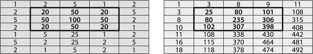
Figure 6-19. The 7-by-5 image of Figure 6-18 shown numerically at left (with the origin assumed to be the upper-left ) and converted to an integral image at right
[86] This is because we need to put in a buffer of zero values along the x-axis and y-axis in order to make computation efficient.