Cameras and image sensors must usually deal not only with the contrast in a scene but also with the image sensors' exposure to the resulting light in that scene. In a standard camera, the shutter and lens aperture settings juggle between exposing the sensors to too much or too little light. Often the range of contrasts is too much for the sensors to deal with; hence there is a trade-off between capturing the dark areas (e.g., shadows), which requires a longer exposure time, and the bright areas, which require shorter exposure to avoid saturating "whiteouts."
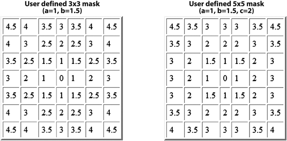
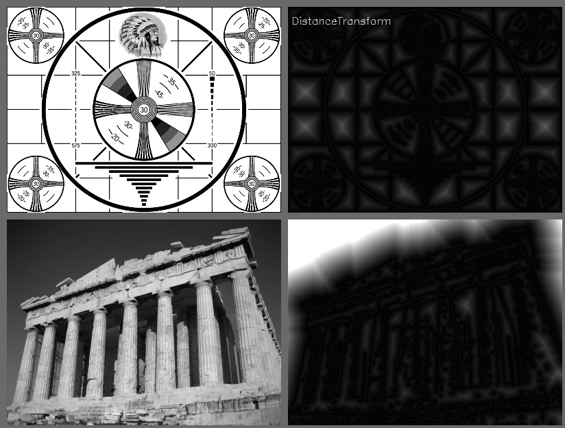
Figure 6-21. First a Canny edge detector was run with param1=100 and param2=200; then the distance transform was run with the output scaled by a factor of 5 to increase visibility
After the picture has been taken, there's nothing we can do about what the sensor recorded; however, we can still take what's there and try to expand the dynamic range of the image. The most commonly used technique for this is histogram equalization. [88][89] In Figure 6-22 we can see that the image on the left is poor because there's not much variation of the range of values. This is evident from the histogram of its intensity values on the right. Because we are dealing with an 8-bit image, its intensity values can range from 0 to 255, but the histogram shows that the actual intensity values are all clustered near the middle of the available range. Histogram equalization is a method for stretching this range out.
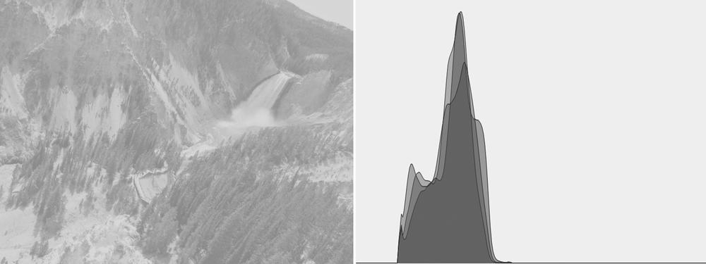
Figure 6-22. The image on the left has poor contrast, as is confirmed by the histogram of its intensity values on the right
The underlying math behind histogram equalization involves mapping one distribution (the given histogram of intensity values) to another distribution (a wider and, ideally, uniform distribution of intensity values). That is, we want to spread out the y-values of the original distribution as evenly as possible in the new distribution. It turns out that there is a good answer to the problem of spreading out distribution values: the remapping function should be the cumulative distribution function. An example of the cumulative density function is shown in Figure 6-23 for the somewhat idealized case of a distribution that was originally pure Gaussian. However, cumulative density can be applied to any distribution; it is just the running sum of the original distribution from its negative to its positive bounds.
We may use the cumulative distribution function to remap the original distribution as an equally spread distribution (see Figure 6-24) simply by looking up each y-value in the original distribution and seeing where it should go in the equalized distribution.

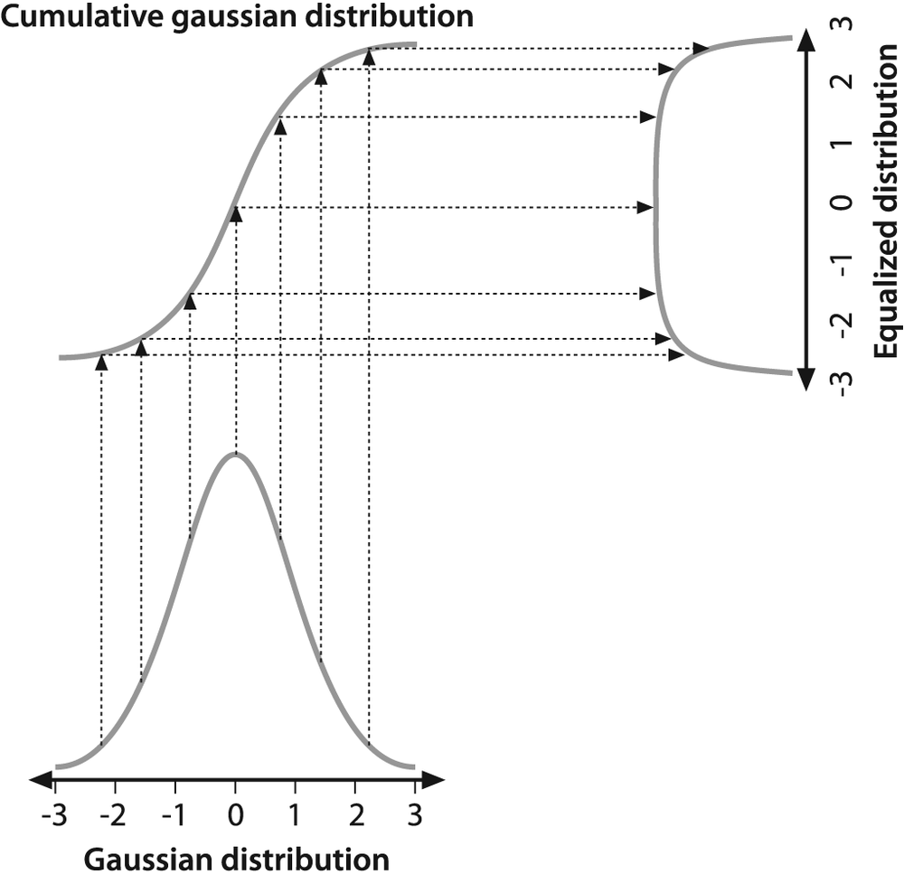
For continuous distributions the result will be an exact equalization, but for digitized/discrete distributions the results may be far from uniform.
Applying this equalization process to Figure 6-22 yields the equalized intensity distribution histogram and resulting image in Figure 6-25. This whole process is wrapped up in one neat function:
void cvEqualizeHist(
  const CvArr* src,
  CvArr*       dst
);
In cvEqualizeHist(), the source and destination must
be single-channel, 8-bit images of the same size. For color images you will have to separate
the channels and process them one by one.
[88] If you are wondering why histogram equalization is not in the chapter on histograms (Chapter 7), the reason is that histogram equalization makes no explicit use of any histogram data types. Although histograms are used internally, the function (from the user's perspective) requires no histograms at all.
[89] Histogram equalization is an old mathematical technique; its use in image processing is described in various textbooks [Jain86; Russ02; Acharya05], conference papers [Schwarz78], and even in biological vision [Laughlin81].