We are finally ready to start talking about contours. To start
with, we should define exactly what a contour is. A contour is a list of points that
represent, in one way or another, a curve in an image. This representation can be different
depending on the circumstance at hand. There are many ways to represent a curve. Contours
are represented in OpenCV by sequences in which every entry in the sequence encodes
information about the location of the next point on the curve. We will dig into the details
of such sequences in a moment, but for now just keep in mind that a contour is represented
in OpenCV by a CvSeq sequence that is, one way or
another, a sequence of points.
The function cvFindContours() computes contours from
binary images. It can take images created by cvCanny(),
which have edge pixels in them, or images created by functions like cvThreshold() or cvAdaptiveThreshold(), in
which the edges are implicit as boundaries between positive and negative regions.[108]
Before getting to the function prototype, it is worth taking a moment to understand
exactly what a contour is. Along the way, we will encounter the concept of a contour tree,
which is important for understanding how cvFindContours()
(retrieval methods derive from Suzuki [Suzuki85]) will communicate its results to us.
Take a moment to look at Figure 8-2,
which depicts the functionality of cvFindContours(). The
upper part of the figure shows a test image containing a number of white regions (labeled A
through E) on a dark background.[109] The lower portion of the figure depicts the same image along with the contours
that will be located by cvFindContours(). Those contours
are labeled cX or hX, where "c" stands for "contour", "h" stands for "hole", and "X" is some
number. Some of those contours are dashed lines; they represent exterior
boundaries of the white regions (i.e., nonzero regions). OpenCV and cvFindContours() distinguish between these exterior boundaries
and the dotted lines, which you may think of either as interior
boundaries or as the exterior boundaries of holes (i.e.,
zero regions).
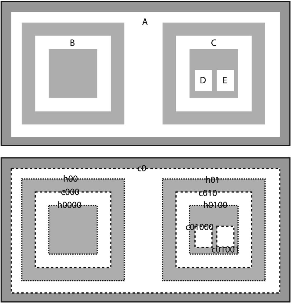
Figure 8-2. A test image (above) passed to cvFindContours() (below): the found contours may be either of two types, exterior "contours" (dashed lines) or "holes" (dotted lines)
The concept of containment here is important in many applications. For this reason, OpenCV can be asked to assemble the found contours into a contour tree[110] that encodes the containment relationships in its structure. A contour tree corresponding to this test image would have the contour called c0 at the root node, with the holes h00 and h01 as its children. Those would in turn have as children the contours that they directly contain, and so on.
Tip
It is interesting to note the consequences of using cvFindContours() on an image generated by cvCanny() or a similar edge detector relative to what happens with a binary
image such as the test image shown in Figure 8-2. Deep down, cvFindContours() does not really know anything about edge
images. This means that, to cvFindContours(), an "edge"
is just a very thin "white" area. As a result, for every exterior contour there will be a
hole contour that almost exactly coincides with it. This hole is actually just inside of
the exterior boundary. You can think of it as the white-to-black transition that marks the
interior edge of the edge.
Now it's time to look at the cvFindContours()
function itself: to clarify exactly how we tell it what we want and how we interpret its
response.
int cvFindContours(
  IplImage*              img,
  CvMemStorage*          storage,
  CvSeq**                firstContour,
  int                    headerSize  = sizeof(CvContour),
  CvContourRetrievalMode mode        = CV_RETR_LIST,
  CvChainApproxMethod    method      = CV_CHAIN_APPROX_SIMPLE
);
The first argument is the input image; this image should be an 8-bit single-channel
image and will be interpreted as binary (i.e., as if all nonzero pixels are equivalent to
one another). When it runs, cvFindContours() will
actually use this image as scratch space for computation, so if you need that image for
anything later you should make a copy and pass that to cvFindContours(). The next argument, storage, indicates a place where cvFindContours() can find memory in which to record the contours. This storage
area should have been allocated with cvCreateMemStorage(), which we covered earlier in the chapter. Next is firstContour, which is a pointer to a CvSeq*. The function cvFindContours() will
allocate this pointer for you, so you shouldn't allocate it yourself. Instead, just pass in
a pointer to that pointer so that it can be set by the function. No allocation/de-allocation
(new/delete or malloc/free) is needed. It is at this location (i.e., *firstContour) that you will find a pointer to the head of the
constructed contour tree.[111] The return value of cvFindContours() is the
total number of contours found.
CvSeq* firstContour = NULL;
cvFindContours( ..., &firstContour, ... );
The headerSize is just telling cvFindContours() more about the objects that it will be
allocating; it can be set to sizeof(CvContour) or to
sizeof(CvChain) (the latter is used when the
approximation method is set to CV_CHAIN_CODE).[112] Finally, we have the mode and method, which (respectively) further clarify exactly
what is to be computed and how it is to be
computed.
The mode variable can be set to any of four options:
CV_RETR_EXTERNAL, CV_RETR_LIST, CV_RETR_CCOMP, or
CV_RETR_TREE. The value of mode indicates to cvFindContours() exactly
what contours we would like found and how we would like the result presented to us. In
particular, the manner in which the tree node variables (h_prev,
h_next, v_prev, and v_next) are used to "hook
up" the found contours is determined by the value of mode. In Figure 8-3, the
resulting topologies are shown for all four possible values of mode. In every case, the structures can be thought of as "levels" which are
related by the "horizontal" links (h_next and h_prev), and those levels are separated from one another by the
"vertical" links (v_next and v_prev).
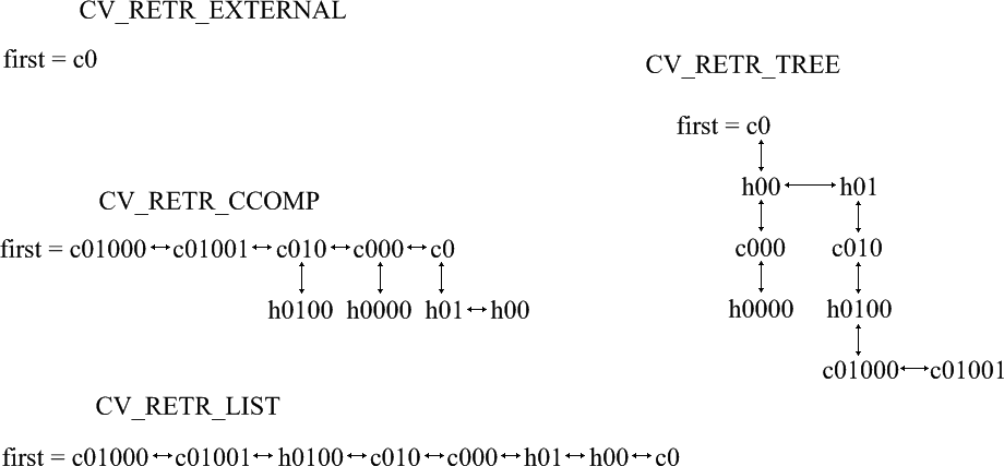
Figure 8-3. The way in which the tree node variables are used to "hook up" all of the contours located by cvFindContours()
-
CV_RETR_EXTERNAL Retrieves only the extreme outer contours. In Figure 8-2, there is only one exterior contour, so Figure 8-3 indicates the first contour points to that outermost sequence and that there are no further connections.
-
CV_RETR_LIST Retrieves all the contours and puts them in the list. Figure 8-3 depicts the list resulting from the test image in Figure 8-2. In this case, eight contours are found and they are all connected to one another by
h_prevandh_next (v_prevandv_nextare not used here.)-
CV_RETR_CCOMP Retrieves all the contours and organizes them into a two-level hierarchy, where the top-level boundaries are external boundaries of the components and the second-level boundaries are boundaries of the holes. Referring to Figure 8-3, we can see that there are five exterior boundaries, of which three contain holes. The holes are connected to their corresponding exterior boundaries by
v_nextandv_prev. The outermost boundary c0 contains two holes. Becausev_nextcan contain only one value, the node can only have one child. All of the holes inside of c0 are connected to one another by theh_prevandh_nextpointers.-
CV_RETR_TREE Retrieves all the contours and reconstructs the full hierarchy of nested contours. In our example (Figures Figure 8-2 and Figure 8-3), this means that the root node is the outermost contour c0. Below c0 is the hole h00, which is connected to the other hole h01 at the same level. Each of those holes in turn has children (the contours c000 and c010, respectively), which are connected to their parents by vertical links. This continues down to the most-interior contours in the image, which become the leaf nodes in the tree.
The next five values pertain to the method (i.e., how
the contours are approximated).
-
CV_CHAIN_CODE Outputs contours in the Freeman chain code;[113] all other methods output polygons (sequences of vertices).[114]
-
CV_CHAIN_APPROX_NONE Translates all the points from the chain code into points.
-
CV_CHAIN_APPROX_SIMPLE Compresses horizontal, vertical, and diagonal segments, leaving only their ending points.
CV_CHAIN_APPROX_TC89_L1orCV_CHAIN_APPROX_TC89_KCOSApplies one of the flavors of the Teh-Chin chain approximation algorithm.
-
CV_LINK_RUNS Completely different algorithm (from those listed above) that links horizontal segments of 1s; the only retrieval mode allowed by this method is
CV_RETR_LIST.
As you can see, there is a lot to sequences and contours. The good news is that, for
our current purpose, we need only a small amount of what's available. When cvFindContours() is called, it will give us a bunch of
sequences. These sequences are all of one specific type; as we saw, which particular type
depends on the arguments passed to cvFindContours().
Recall that the default mode is CV_RETR_LIST and the
default method is CV_CHAIN_APPROX_SIMPLE.
These sequences are sequences of points; more precisely, they are contours'the actual topic of this chapter. The key thing to remember about contours is that they are just a special case of sequences.[115] In particular, they are sequences of points representing some kind of curve in (image) space. Such a chain of points comes up often enough that we might expect special functions to help us manipulate them. Here is a list of these functions.
int cvFindContours(
  CvArr*        image,
  CvMemStorage* storage,
  CvSeq**       first_contour,
  int           header_size   = sizeof(CvContour),
  int           mode          = CV_RETR_LIST,
  int           method        = CV_CHAIN_APPROX_SIMPLE,
  CvPoint       offset        = cvPoint(0,0)
);
CvContourScanner cvStartFindContours(
  CvArr*        image,
  CvMemStorage* storage,
  int           header_size   = sizeof(CvContour),
  int           mode          = CV_RETR_LIST,
  int           method        = CV_CHAIN_APPROX_SIMPLE,
  CvPoint       offset        = cvPoint(0,0)
);
CvSeq* cvFindNextContour(
  CvContourScanner scanner
);
void cvSubstituteContour(
  CvContourScanner scanner,
  CvSeq*           new_contour
);
CvSeq* cvEndFindContour(
  CvContourScanner* scanner
);
CvSeq* cvApproxChains(
  CvSeq*        src_seq,
  CvMemStorage* storage,
  int           method            = CV_CHAIN_APPROX_SIMPLE,
  double        parameter         = 0,
  int           minimal_perimeter = 0,
  int           recursive         = 0
);
First is the cvFindContours() function, which we
encountered earlier. The second function, cvStartFindContours(), is closely related to cvFindContours() except that it is used when you want the contours one at a
time rather than all packed up into a higher-level structure (in the manner of cvFindContours()). A call to cvStartFindContours() returns a CvSequenceScanner. The scanner contains some simple state information about
what has and what has not been read out.[116] You can then call cvFindNextContour() on
the scanner to successively retrieve all of the contours found. A NULL return means that no more contours are left.
cvSubstituteContour() allows the contour to which a
scanner is currently pointing to be replaced by some other contour. A useful
characteristic of this function is that, if the new_contour argument is set to NULL, then
the current contour will be deleted from the chain or tree to which the scanner is
pointing (and the appropriate updates will be made to the internals of the affected
sequence, so there will be no pointers to nonexistent objects).
Finally, cvEndFindContour() ends the scanning and
sets the scanner to a "done" state. Note that the sequence the scanner was scanning is not
deleted; in fact, the return value of cvEndFindContour() is a pointer to the first element in the
sequence.
The final function is cvApproxChains(). This
function converts Freeman chains to polygonal representations (precisely or with some
approximation). We will discuss cvApproxPoly() in
detail later in this chapter (see the section "Polygon Approximations").
Normally, the contours created by cvFindContours()
are sequences of vertices (i.e., points). An alternative representation can be generated
by setting the method to CV_CHAIN_CODE. In this case,
the resulting contours are stored internally as Freeman chains
[Freeman67] (Figure 8-4). With a Freeman
chain, a polygon is represented as a sequence of steps in one of eight directions; each
step is designated by an integer from 0 to 7. Freeman chains have useful applications in
recognition and other contexts. When working with Freeman chains, you can read out their
contents via two "helper" functions:
void cvStartReadChainPoints(
   CvChain*         chain,
   CvChainPtReader* reader
);
CvPoint cvReadChainPoint(
   CvChainPtReader* reader
);
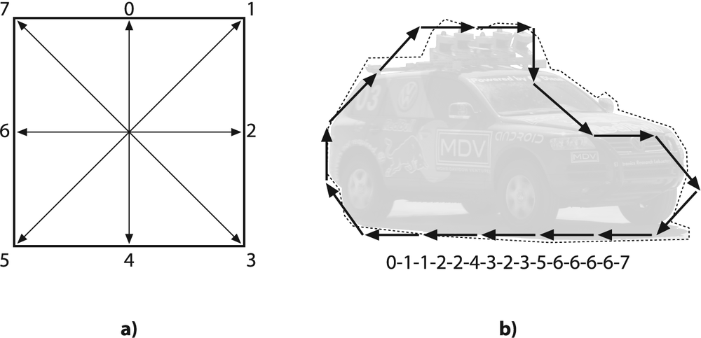
Figure 8-4. Panel a, Freeman chain moves are numbered 0-7; panel b, contour converted to a Freeman chain-code representation starting from the back bumper
The first function takes a chain as its argument and the second function is a chain
reader. The CvChain structure is a form of CvSeq.[117] Just as CvContourScanner iterates through
different contours, CvChainPtReader iterates through a
single contour represented by a chain. In this respect, CvChainPtReader is similar to the more general CvSeqReader, and cvStartReadChainPoints
plays the role of cvStartReadSeq. As you might expect,
CvChainPtReader returns NULL when there's nothing left to read.
One of our most basic tasks is drawing a contour on the screen. For this we have
cvDrawContours():
void  cvDrawContours(
   CvArr*   img,
   CvSeq*   contour,
   CvScalar external_color,
   CvScalar hole_color,
   int      max_level,
   int      thickness     = 1,
   int      line_type     = 8,
   CvPoint  offset        = cvPoint(0,0)
);
The first argument is simple: it is the image on which to draw the contours. The next
argument, contour, is not quite as simple as it looks.
In particular, it is really treated as the root node of a contour tree. Other arguments
(primarily max_level) will determine what is to be done
with the rest of the tree. The next argument is pretty straightforward: the color with
which to draw the contour. But what about hole_color?
Recall that OpenCV distinguishes between contours that are exterior contours and those
that are hole contours (the dashed and dotted lines, respectively, in Figure 8-2). When drawing either a single
contour or all contours in a tree, any contour that is marked as a "hole" will be drawn in
this alternative color.
The max_level tells cvDrawContours() how to handle any contours that might be attached to
contour by means of the node tree variables. This
argument can be set to indicate the maximum depth to traverse in the drawing. Thus,
max_level=0 means that all the contours on the same
level as the input level (more exactly, the input contour and the contours next to it) are
drawn, max_level=1 means that all the contours on the
same level as the input and their children are drawn, and so forth. If the contours in
question were produced by cvFindContours() using either
CV_RETR_CCOMP or CV_RETR_TREE mode, then the additional idiom of negative values for max_level is also supported. In this case, max_level=-1 is interpreted to mean that only the input
contour will be drawn, max_level=-2 means that the
input contour and its direct children will the drawn, and so on. The
sample code in …/opencv/samples/c/contours.c
illustrates this point.
The parameters thickness and line_type have their usual meanings.[118] Finally, we can give an offset to the draw
routine so that the contour will be drawn elsewhere than at the absolute coordinates by
which it was defined. This feature is particularly useful when the contour has already
been converted to center-of-mass or other local coordinates.
More specifically, offset would be helpful if we
ran cvFindContours() one or more times in different
image subregions (ROIs) and thereafter wanted to display all the results within the
original large image. Conversely, we could use offset
if we'd extracted a contour from a large image and then wanted to form a small mask for
this contour.
Our Example 8-2 is drawn from the OpenCV package. Here we create a window with an image in it. A trackbar sets a simple threshold, and the contours in the thresholded image are drawn. The image is updated whenever the trackbar is adjusted.
Example 8-2. Finding contours based on a trackbar's location; the contours are updated whenever the trackbar is moved
#include <cv.h>
#include <highgui.h>

IplImage*      g_image    = NULL;
IplImage*      g_gray    = NULL;
int            g_thresh  = 100;
CvMemStorage*  g_storage  = NULL;

void on_trackbar(int) {
  if( g_storage==NULL ) {
    g_gray = cvCreateImage( cvGetSize(g_image), 8, 1 );
    g_storage = cvCreateMemStorage(0);
  } else {
    cvClearMemStorage( g_storage );
  }
  CvSeq* contours = 0;
  cvCvtColor( g_image, g_gray, CV_BGR2GRAY );
  cvThreshold( g_gray, g_gray, g_thresh, 255, CV_THRESH_BINARY );
  cvFindContours( g_gray, g_storage, &contours );
  cvZero( g_gray );
  if( contours )
    cvDrawContours(
      g_gray,
      contours,
      cvScalarAll(255),
      cvScalarAll(255),
      100
    );
  cvShowImage( "Contours", g_gray );
}

int main( int argc, char** argv )
{
  if( argc != 2 || !(g_image = cvLoadImage(argv[1])) )
  return -1;
  cvNamedWindow( "Contours", 1 );
  cvCreateTrackbar(
    "Threshold",
    "Contours",
    &g_thresh,
    255,
    on_trackbar
  );
  on_trackbar(0);
  cvWaitKey();
  return 0;
}
Here, everything of interest to us is happening inside of the function on_trackbar(). If the global variable g_storage is still at its (NULL) initial
value, then cvCreateMemStorage(0) creates the memory
storage and g_gray is initialized to a blank image the
same size as g_image but with only a single channel. If
g_storage is non-NULL, then we've been here before and thus need only empty the storage so it
can be reused. On the next line, a CvSeq* pointer is
created; it is used to point to the sequence that we will create via cvFindContours().
Next, the image g_image is converted to grayscale
and thresholded such that only those pixels brighter than g_thresh are retained as nonzero. The cvFindContours() function is then called on this thresholded image. If any
contours were found (i.e., if contours is non-NULL), then cvDrawContours() is called and the contours are drawn (in white) onto the
grayscale image.
[108] There are some subtle differences between passing edge images and binary images to
cvFindContours(); we will discuss those
shortly.
[109] For clarity, the dark areas are depicted as gray in the figure, so simply imagine
that this image is thresholded such that the gray areas are set to black before passing
to cvFindContours().
[110] Contour trees first appeared in Reeb [Reeb46] and were further developed by [Bajaj97], [Kreveld97], [Pascucci02], and [Carr04].
[111] As we will see momentarily, contour trees are just one way that cvFindContours() can organize the contours it finds. In any case, they will
be organized using the CV_TREE_NODE_FIELDS elements
of the contours that we introduced when we first started talking about sequences.
[112] In fact, headerSize can be an arbitrary number
equal to or greater than the values listed.
[113] Freeman chain codes will be discussed in the section entitled "Contours Are Sequences".
[114] Here "vertices" means points of type CvPoint. The sequences created by cvFindContours() are the same as those created with cvCreateSeq() with the flag CV_SEQ_ELTYPE_POINT. (That function and flag will be described in
detail later in this chapter.)
[115] OK, there's a little more to it than this, but we did not want to be sidetracked
by technicalities and so will clarify in this footnote. The type CvContour is not identical to CvSeq. In the way such things are handled in OpenCV, CvContour is, in effect, derived from CvSeq. The CvContour
type has a few extra data members, including a color and a CvRect for stashing its bounding box.
[116] It is important not to confuse a CvSequenceScanner with the similarly named CvSeqReader. The latter is for reading the elements in a sequence,
whereas the former is used to read from what is, in effect, a list of
sequences.
[117] You may recall a previous mention of "extensions" of the CvSeq structure; CvChain is such an
extension. It is defined using the CV_SEQUENCE_FIELDS() macro and has one extra element in it, a CvPoint representing the origin. You can think of CvChain as being "derived from" CvSeq. In this sense, even though the return type of cvApproxChains() is indicated as CvSeq*, it is really a pointer to a chain and is not a normal
sequence.
[118] In particular, thickness=-1 (aka CV_FILLED) is useful for converting the contour tree (or
an individual contour) back to the black-and-white image from which it was extracted.
This feature, together with the offset parameter,
can be used to do some quite complex things with contours: intersect and merge
contours, test points quickly against the contours, perform morphological operations
(erode/dilate), etc.