When analyzing an image, there are many different things we might want to do with contours. After all, most contours are—or are candidates to be—things that we are interested in identifying or manipulating. The various relevant tasks include characterizing the contours in various ways, simplifying or approximating them, matching them to templates, and so on.
In this section we will examine some of these common tasks and visit the various functions built into OpenCV that will either do these things for us or at least make it easier for us to perform our own tasks.
If we are drawing a contour or are engaged in shape analysis, it is common to
approximate a contour representing a polygon with another contour having fewer vertices.
There are many different ways to do this; OpenCV offers an implementation of one of
them.[119] The routine cvApproxPoly() is an
implementation of this algorithm that will act on a sequence of contours:
CvSeq*  cvApproxPoly(
   const void*   src_seq,
   int           header_size,
   CvMemStorage* storage,
   int           method,
   double        parameter,
   int           recursive  = 0
);
We can pass a list or a tree sequence containing contours to cvApproxPoly(), which will then act on all of the contained contours. The
return value of cvApproxPoly() is actually just the
first contour, but you can move to the others by using the h_next (and v_next, as appropriate)
elements of the returned sequence.
Because cvApproxPoly() needs to create the objects
that it will return a pointer to, it requires the usual CvMemStorage* pointer and header size (which, as usual, is set to sizeof(CvContour)).
The method argument is always set to CV_POLY_APPROX_DP (though other algorithms could be selected
if they become available). The next two arguments are specific to the method (of which,
for now, there is but one). The parameter argument is
the precision parameter for the algorithm. To understand how this parameter works, we must
take a moment to review the actual algorithm.[120] The last argument indicates whether the algorithm should (as mentioned
previously) be applied to every contour that can be reached via the h_next and v_next pointers.
If this argument is 0, then only the contour directly pointed to by src_seq will be approximated.
So here is the promised explanation of how the algorithm works. In Figure 8-5, starting with a contour (panel b), the algorithm begins by picking two extremal points and connecting them with a line (panel c). Then the original polygon is searched to find the point farthest from the line just drawn, and that point is added to the approximation.
The process is iterated (panel d), adding the next most distant point to the accumulated approximation, until all of the points are less than the distance indicated by the precision parameter (panel f). This means that good candidates for the parameter are some fraction of the contour's length, or of the length of its bounding box, or a similar measure of the contour's overall size.
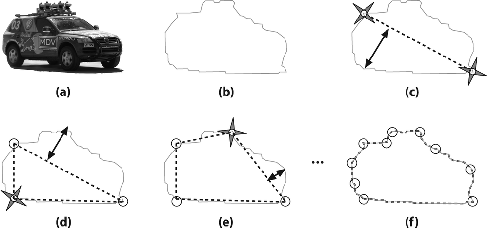
Figure 8-5. Visualization of the DP algorithm used by cvApproxPoly(): the original image (a) is approximated by a contour (b) and then, starting from the first two maximally separated vertices (c), the additional vertices are iteratively selected from that contour (d)-(f)
Closely related to the approximation just described is the process of finding
dominant points. A dominant point is defined as a point
that has more information about the curve than do other points. Dominant points are used
in many of the same contexts as polygon approximations. The routine cvFindDominantPoints() implements what is known as the
IPAN[121] [Chetverikov99] algorithm.
CvSeq* cvFindDominantPoints(
   CvSeq*        contour,
   CvMemStorage* storage,
   int           method      = CV_DOMINANT_IPAN,
   double        parameter1  = 0,
   double        parameter2  = 0,
   double        parameter3  = 0,
   double        parameter4  = 0
);
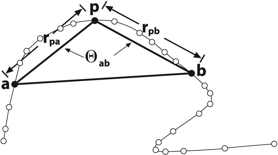
In essence, the IPAN algorithm works by scanning along the contour and trying to construct triangles on the interior of the curve using the available vertices. That triangle is characterized by its size and the opening angle (see Figure 8-6). The points with large opening angles are retained provided that their angles are smaller than a specified global threshold and smaller than their neighbors.
The routine cvFindDominantPoints() takes the usual
CvSeq* and CvMemStorage* arguments. It also requires a method, which (as with cvApproxPoly()) can
take only one argument at this time: CV_DOMINANT_IPAN.
The next four arguments are: a minimal distance dmin, a maximal distance dmax, a neighborhood distance dn, and a maximum angle θmax. As shown in Figure 8-6, the algorithm first constructs all triangles for which rpa and rpb fall between dmin and dmax and for which θab < θmax. This is followed by a second pass in which only those points p with the smallest associated value of θab in the neighborhood dn are retained (the value of dn should never exceed dmax). Typical values for dmin, dmax, dn, and θmax are 7, 9, 9, and 150 (the last argument is an angle and is measured in degrees).
Another task that one often faces with contours is computing their various summary characteristics. These might include length or some other form of size measure of the overall contour. Other useful characteristics are the contour moments, which can be used to summarize the gross shape characteristics of a contour (we will address these in the next section).
The subroutine cvContourPerimeter() will take a
contour and return its length. In fact, this function is actually a macro for the
somewhat more general cvArcLength().
double  cvArcLength(
   const void* curve,
   CvSlice     slice     = CV_WHOLE_SEQ,
   int         is_closed = -1
);
#define cvContourPerimeter( contour )             \
  cvArcLength( contour, CV_WHOLE_SEQ, 1 )
The first argument of cvArcLength() is the
contour itself, whose form may be either a sequence of points (CvContour* or CvSeq*) or an
n-by-1 two-channel matrix (CvMat*) of points.
Next are the slice argument and is_closed indicating whether the contour should be treated as closed. The
possible values of is_closed are: "true" (any value greater than
zero), "false" (a value of zero), or a negative value. A negative value (which is the
default) indicates that the function should check the special CV_SEQ_FLAG_CLOSED bit in the sequence header to determine if the sequence
is closed or not. The slice argument allows us to select only some
subset of the points in the curve.[122]
Closely related to cvArcLegth() is cvContourArea(), which (as its name suggests) computes the
area of a contour. It takes the contour as an argument and the same slice argument as
cvArcLength().
double  cvContourArea(
   const CvArr* contour,
   CvSlice      slice  = CV_WHOLE_SEQ
);
Of course the length and area are simple characterizations of a contour. The next level of detail might be to summarize them with a bounding box or bounding circle or ellipse. There are two ways to do the former, and there is a single method for doing each of the latter.
CvRect  cvBoundingRect(
  CvArr* points,
  int update              = 0
);
CvBox2D  cvMinAreaRect2(
   const CvArr* points,
   CvMemStorage* storage  = NULL
);
The simplest technique is to call cvBoundingRect(); it will return a CvRect that bounds the contour. The points used for the first argument can
be either a contour (CvContour*) or an
n-by-1, two-channel matrix (CvMat*) containing the points in the sequence. To understand the second
argument, update, we must harken back to one of the
earlier footnotes in this chapter. Remember that CvContour is not exactly the same as CvSeq; it does everything CvSeq does but
also a little bit more. One of those CvContour extras
is a CvRect member for referring to its own bounding
box. If you call cvBoundingRect() with update set to 0 then you will just get the contents of that
data member; but if you call with update set to 1,
the bounding box will be computed (and the associated data member will also be
updated).
One problem with the bounding rectangle from cvBoundingRect() is that it is a CvRect
and so can only represent a rectangle whose sides are oriented horizontally and
vertically. In contrast, the routine cvMinAreaRect2()
returns the minimal rectangle that will bound your contour, and this rectangle may be
inclined relative to the vertical; see Figure 8-7. The arguments are otherwise
similar to cvBoundingRect(). The OpenCV data type
CvBox2D is just what is needed to represent such a
rectangle.
typedef struct  CvBox2D {
  CvPoint2D32f center;
  CvSize2D32f  size;
  float         angle;
} CvBox2D;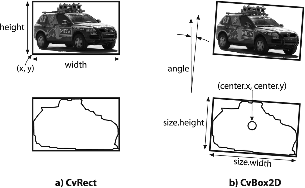
Next we have cvMinEnclosingCircle().[123] This routine works pretty much the same as the bounding box routines, with the same flexibility of being able to set
points to be either a sequence or an array of
two-dimensional points.
int  cvMinEnclosingCircle(
   const CvArr*  points,
   CvPoint2D32f* center,
   float*        radius
);
There is no special structure in OpenCV for representing circles, so we need to pass
in pointers for a center point and a floating-point
variable radius that can be used by cvMinEnclosingCircle() to report the results of its
computations.
As with the minimal enclosing circle, OpenCV also provides a method for fitting an ellipse to a set of points:
CvBox2D cvFitEllipse2(
  const CvArr* points
);
The subtle difference between cvMinEnclosingCircle() and cvFitEllipse2() is that the former simply computes the smallest circle that
completely encloses the given contour, whereas the latter uses a fitting function and
returns the ellipse that is the best approximation to the contour. This means that not
all points in the contour will be enclosed in the ellipse returned by cvFitEllipse2(). The fitting is done using a least-squares
fitness function.
The results of the fit are returned in a CvBox2D
structure. The indicated box exactly encloses the ellipse. See Figure 8-8.

When dealing with bounding boxes and other summary representations of polygon contours, it is often desirable to perform such simple geometrical checks as polygon overlap or a fast overlap check between bounding boxes. OpenCV provides a small but handy set of routines for this sort of geometrical checking.
CvRect cvMaxRect(
    const CvRect* rect1,
    const CvRect* rect2
);
void cvBoxPoints(
    CvBox2D       box,
    CvPoint2D32f  pt[4]
);
CvSeq* cvPointSeqFromMat(
    int           seq_kind,
    const CvArr*  mat,
    CvContour*    contour_header,
    CvSeqBlock*   block
);
double cvPointPolygonTest(
    const CvArr*  contour,
    CvPoint2D32f  pt,
    int           measure_dist
);
The first of these functions, cvMaxRect(), computes
a new rectangle from two input rectangles. The new rectangle is the smallest rectangle
that will bound both inputs.
Next, the utility function cvBoxPoints() simply
computes the points at the corners of a CvBox2D
structure. You could do this yourself with a bit of trigonometry, but you would soon grow
tired of that. This function does this simple pencil pushing for you.
The third utility function, cvPointSeqFromMat(),
generates a sequence structure from a matrix. This is useful when you want to use a
contour function that does not also take matrix arguments. The input to cvPointSeqFromMat() first requires you to indicate what sort
of sequence you would like. The variable seq_kind may
be set to any of the following: zero (0), indicating
just a point set; CV_SEQ_KIND_CURVE, indicating that
the sequence is a curve; or CV_SEQ_KIND_CURVE |
CV_SEQ_FLAG_CLOSED, indicating that the sequence is a closed curve. Next you
pass in the array of points, which should be an n-by-1 array of
points. The points should be of type CV_32SC2 or
CV_32FC2 (i.e., they should be single-column,
two-channel arrays). The next two arguments are pointers to values that will be computed
by cvPointSeqFromMat(), and contour_header is a contour structure that you should already have created
but whose internals will be filled by the function call. This is similarly the case for
block, which will also be filled for you.[124] Finally the return value is a CvSeq*
pointer, which actually points to the very contour structure you passed in yourself. This
is a convenience, because you will generally need the sequence address when calling the
sequence-oriented functions that motivated you to perform this conversion in the first
place.
The last geometrical tool-kit function to be presented here is cvPointPolygonTest(), a function that allows you to test
whether a point is inside a polygon (indicated by a sequence). In particular, if the
argument measure_dist is nonzero then the function
returns the distance to the nearest contour edge; that distance is 0 if the point is
inside the contour and positive if the point is outside. If the measure_dist argument is 0 then the return values are simply + 1, – 1, or 0
depending on whether the point is inside, outside, or on an edge (or vertex),
respectively. The contour itself can be either a sequence or an
n-by-1 two-channel matrix of points.
[119] For aficionados, the method used by OpenCV is the Douglas-Peucker (DP) approximation [Douglas73]. Other popular methods are the Rosenfeld-Johnson [Rosenfeld73] and Teh-Chin [Teh89] algorithms.
[120] If that's too much trouble, then just set this parameter to a small fraction of the total curve length.
[121] For "Image and Pattern Analysis Group," Hungarian Academy of Sciences. The algorithm is often referred to as "IPAN99" because it was first published in 1999.
[122] Almost always, the default value CV_WHOLE_SEQ
is used. The structure CvSlice contains only two
elements: start_index and end_index. You can create your own slice to put here
using the helper constructor function cvSlice (int start,
int end). Note that CV_WHOLE_SEQ is
just shorthand for a slice starting at 0 and ending at some very large
number.
[123] For more information on the inner workings of these fitting techniques, see Fitzgibbon and Fisher [Fitzgibbon95] and Zhang [Zhang96].
[124] You will probably never use block. It exists
because no actual memory is copied when you call cvPoint
SeqFromMat(); instead, a "virtual" memory block is created that actually
points to the matrix you yourself provided. The variable block is used to create a
reference to that memory of the kind expected by internal sequence or contour
calculations.