Delaunay Triangulation, Voronoi Tesselation

Delaunay triangulation is a technique invented in 1934 [Delaunay34] for connecting points in a space into triangular groups such that the minimum angle of all the angles in the triangulation is a maximum. This means that Delaunay triangulation tries to avoid long skinny triangles when triangulating points. See Figure 9-12 to get the gist of triangulation, which is done in such a way that any circle that is fit to the points at the vertices of any given triangle contains no other vertices. This is called the circum-circle property (panel c in the figure).

For computational efficiency, the Delaunay algorithm invents a far-away outer bounding triangle from which the algorithm starts. Figure 9-12(b) represents the fictitious outer triangle by dotted lines going out to its vertex. Figure 9-12(c) shows some examples of the circum-circle property, including one of the circles linking two outer points of the real data to one of the vertices of the fictitious external triangle.

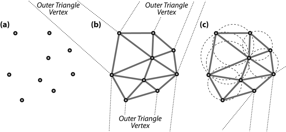
Figure 9-12. Delaunay triangulation: (a) set of points; (b) Delaunay triangulation of the point set with trailers to the outer bounding triangle; (c) example circles showing the circum-circle property

There are now many algorithms to compute Delaunay triangulation; some are very efficient but with difficult internal details. The gist of one of the more simple algorithms is as follows:

1. Add the external triangle.

2. Add an internal point; then search over all the triangles' circum-circles containing that point and remove those triangulations.

3. Re-triangulate the graph, including the new point in the circum-circles of the just removed triangulations.

4. Return to step 2 until there are no more points to add.

The order of complexity of this algorithm is O(n2) in the number of data points. The best algorithms are (on average) as low as O(n log log n).

Great—but what is it good for? For one thing, remember that this algorithm started with a fictitious outer triangle and so all the real outside points are actually connected to two of that triangle's vertices. Now recall the circum-circle property: circles that are fit through any two of the real outside points and to an external fictitious vertex contain no other inside points. This means that a computer may directly look up exactly which real points form the outside of a set of points by looking at which points are connected to the three outer fictitious vertices. In other words, we can find the convex hull of a set of points almost instantly after a Delaunay triangulation has been done.

We can also find who "owns" the space between points, that is, which coordinates are nearest neighbors to each of the Delaunay vertex points. Thus, using Delaunay triangulation of the original points, you can immediately find the nearest neighbor to a new point. Such a partition is called a Voronoi tessellation (see Figure 9-13). This tessellation is the dual image of the Delaunay triangulation, because the Delaunay lines define the distance between existing points and so the Voronoi lines "know" where they must intersect the Delaunay lines in order to keep equal distance between points. These two methods, calculating the convex hull and nearest neighbor, are important basic operations for clustering and classifying points and point sets.

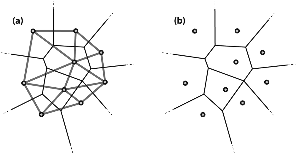
Figure 9-13. Voronoi tessellation, whereby all points within a given Voronoi cell are closer to their Delaunay point than to any other Delaunay point: (a) the Delaunay triangulation in bold with the corresponding Voronoi tessellation in fine lines; (b) the Voronoi cells around each Delaunay point

If you're familiar with 3D computer graphics, you may recognize that Delaunay triangulation is often the basis for representing 3D shapes. If we render an object in three dimensions, we can create a 2D view of that object by its image projection and then use the 2D Delaunay triangulation to analyze and identify this object and/or compare it with a real object. Delaunay triangulation is thus a bridge between computer vision and computer graphics. However, one deficiency of OpenCV (soon to be rectified, we hope; see Chapter 14) is that OpenCV performs Delaunay triangulation only in two dimensions. If we could triangulate point clouds in three dimensions—say, from stereo vision (see Chapter 11)—then we could move seamlessly between 3D computer graphics and computer vision. Nevertheless, 2D Delaunay triangulation is often used in computer vision to register the spatial arrangement of features on an object or a scene for motion tracking, object recognition, or matching views between two different cameras (as in deriving depth from stereo images). Figure 9-14 shows a tracking and recognition application of Delaunay triangulation [Gokturk01; Gokturk02] wherein key facial feature points are spatially arranged according to their triangulation.

Now that we've established the potential usefulness of Delaunay triangulation once given a set of points, how do we derive the triangulation? OpenCV ships with example code for this in the …/opencv/samples/c/delaunay.c file. OpenCV refers to Delaunay triangulation as a Delaunay subdivision, whose critical and reusable pieces we discuss next.

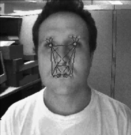
Figure 9-14. Delaunay points can be used in tracking objects; here, a face is tracked using points that are significant in expressions so that emotions may be detected

Creating a Delaunay or Voronoi Subdivision

First we'll need some place to store the Delaunay subdivision in memory. We'll also need an outer bounding box (remember, to speed computations, the algorithm works with a fictitious outer triangle positioned outside a rectangular bounding box). To set this up, suppose the points must be inside a 600-by-600 image:

// STORAGE AND STRUCTURE FOR DELAUNAY SUBDIVISION
//
CvRect        rect = { 0, 0, 600, 600 };  //Our outer bounding box
CvMemStorage* storage;                    //Storage for the Delaunay subdivsion
storage  = cvCreateMemStorage(0);         //Initialize the storage
CvSubdiv2D*    subdiv;                    //The subdivision itself
subdiv = init_delaunay( storage, rect);   //See this function below

The code calls init_delaunay(), which is not an OpenCV function but rather a convenient packaging of a few OpenCV routines:

//INITIALIZATION CONVENIENCE FUNCTION FOR DELAUNAY SUBDIVISION
//
CvSubdiv2D* init_delaunay(
  CvMemStorage* storage,
  CvRect rect
) {
  CvSubdiv2D* subdiv;
  subdiv = cvCreateSubdiv2D(
    CV_SEQ_KIND_SUBDIV2D,
    sizeof(*subdiv),
    sizeof(CvSubdiv2DPoint),
    sizeof(CvQuadEdge2D),
    storage
  );
  cvInitSubdiv Delaunay2D( subdiv, rect ); //rect sets the bounds
  return subdiv;
}

Next we'll need to know how to insert points. These points must be of type float, 32f:

CvPoint2D32f fp;    //This is our point holder

for( i = 0; i < as_many_points_as_you_want; i++ ) {

     // However you want to set points
     //
     fp = your_32f_point_list[i];

     cvSubdivDelaunay2DInsert( subdiv, fp );
}

You can convert integer points to 32f points using the convenience macro cvPoint2D32f(double x, double y) or cvPointTo32f(CvPoint point) located in cxtypes.h. Now that we can enter points to obtain a Delaunay triangulation, we set and clear the associated Voronoi tessellation with the following two commands:

cvCalcSubdiv Voronoi2D( subdiv );  // Fill out Voronoi data in subdiv
cvClearSubdivVoronoi2D( subdiv ); // Clear the Voronoi from subdiv

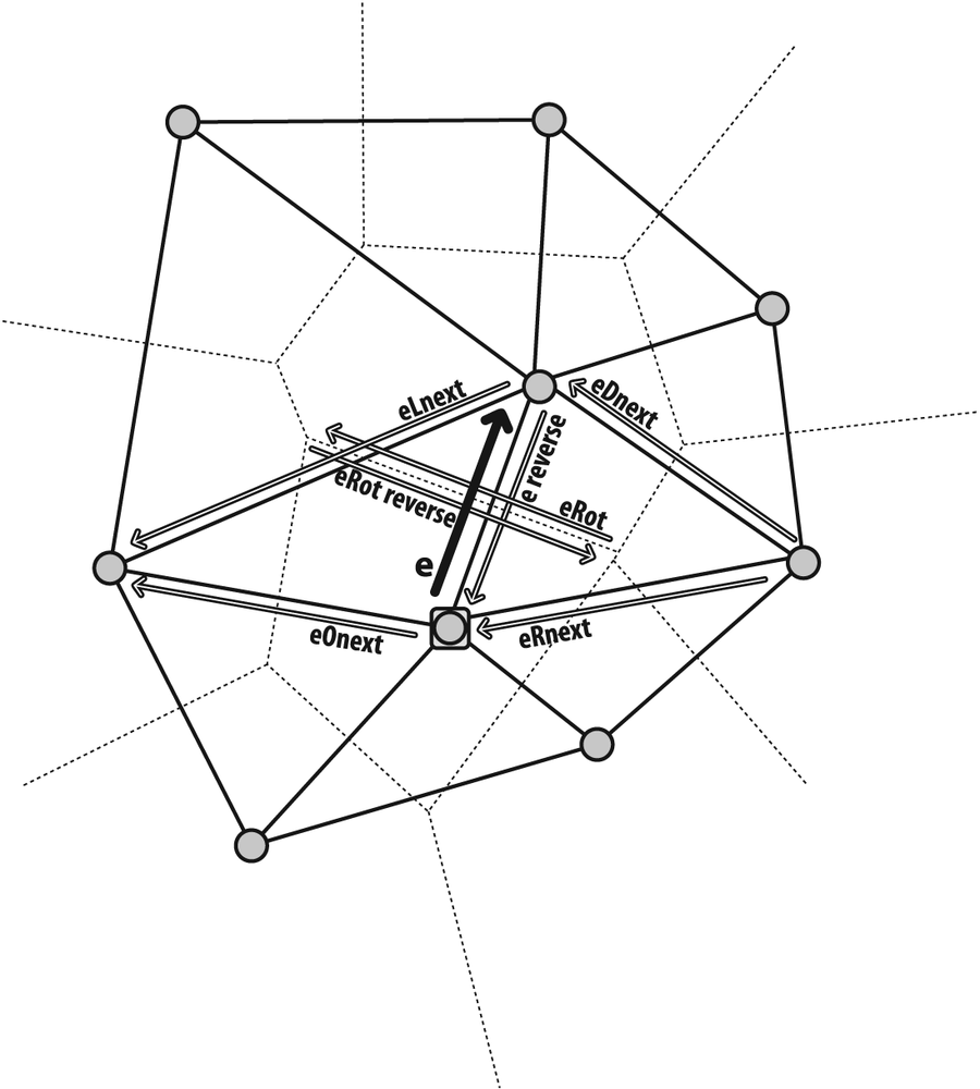
In both functions, subdiv is of type CvSubdiv2D*. We can now create Delaunay subdivisions of two-dimensional point sets and then add and clear Voronoi tessellations to them. But how do we get at the good stuff inside these structures? We can do this by stepping from edge to point or from edge to edge in subdiv; see Figure 9-15 for the basic maneuvers starting from a given edge and its point of origin. We next find the first edges or points in the subdivision in one of two different ways: (1) by using an external point to locate an edge or a vertex; or (2) by stepping through a sequence of points or edges. We'll first describe how to step around edges and points in the graph and then how to step through the graph.

Navigating Delaunay Subdivisions

Figure 9-15 combines two data structures that we'll use to move around on a subdivision graph. The structure cvQuadEdge2D contains a set of two Delaunay and two Voronoi points and their associated edges (assuming the Voronoi points and edges have been calculated with a prior call to cvCalcSubdivVoronoi2D()); see Figure 9-16. The structure CvSubdiv2DPoint contains the Delaunay edge with its associated vertex point, as shown in Figure 9-17. The quad-edge structure is defined in the code following the figure.

Figure 9-15. Edges relative to a given edge, labeled "e", and its vertex point (marked by a square)

// Edges themselves are encoded in long integers. The lower two bits
// are its index (0..3) and upper bits are the quad-edge pointer.
//
typedef long CvSubdiv2DEdge;

// quad-edge structure fields:
//
#define CV_QUADEDGE2D_FIELDS()         /
    int flags;                         /
    struct CvSubdiv2DPoint* pt[4];     /
    CvSubdiv2DEdge  next[4];

typedef struct CvQuadEdge2D {
    CV_QUADEDGE2D_FIELDS()
} CvQuadEdge2D;

The Delaunay subdivision point and the associated edge structure is given by:

#define CV_SUBDIV2D_POINT_FIELDS() /
    int                  flags;    /
     CvSubdiv2DEdge      first;    //*The edge "e" in the figures.*/
     CvPoint2D32f        pt;
     #define CV_SUBDIV2D_VIRTUAL_POINT_FLAG (1 << 30)

     typedef struct CvSubdiv2DPoint
     {
         CV_SUBDIV2D_POINT_FIELDS()
     }
     CvSubdiv2DPoint;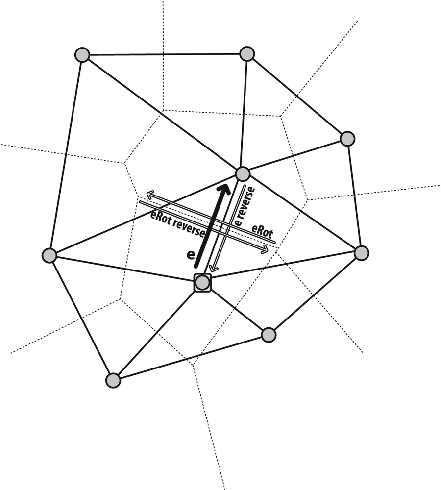

Figure 9-16. Quad edges that may be accessed by cvSubdiv2DRotateEdge() include the Delaunay edge and its reverse (along with their associated vertex points) as well as the related Voronoi edges and points

With these structures in mind, we can now examine the different ways of moving around.

Walking on edges

As indicated by Figure 9-16, we can step around quad edges by using

CvSubdiv2DEdge cvSubdiv2DRotateEdge(
  CvSubdiv2DEdge edge,
  int            type
);

Figure 9-17. A CvSubdiv2DPoint vertex and its associated edge e along with other associated edges that may be accessed via cvSubdiv2DGetEdge()

Given an edge, we can get to the next edge by using the type parameter, which takes one of the following arguments:

• 0, the input edge (e in the figure if e is the input edge)

• 1, the rotated edge (eRot)

• 2, the reversed edge (reversed e)

• 3, the reversed rotated edge (reversed eRot)

Referencing Figure 9-17, we can also get around the Delaunay graph using

CvSubdiv2DEdge cvSubdiv2DGetEdge(
  CvSubdiv2DEdge edge,
  CvNextEdgeType type
);
#define cvSubdiv2DNextEdge( edge ) /
  cvSubdiv2DGetEdge(               /
    edge,                          /
    CV_NEXT_AROUND_ORG             /
  )

Here type specifies one of the following moves:

CV_NEXT_AROUND_ORG

Next around the edge origin (eOnext in Figure 9-17 if e is the input edge)

CV_NEXT_AROUND_DST

Next around the edge vertex (eDnext)

CV_PREV_AROUND_ORG

Previous around the edge origin (reversed eRnext)

CV_PREV_AROUND_DST

Previous around the edge destination (reversed eLnext)

CV_NEXT_AROUND_LEFT

Next around the left facet (eLnext)

CV_NEXT_AROUND_RIGHT

Next around the right facet (eRnext)

CV_PREV_AROUND_LEFT

Previous around the left facet (reversed eOnext)

CV_PREV_AROUND_RIGHT

Previous around the right facet (reversed eDnext)

Note that, given an edge associated with a vertex, we can use the convenience macro cvSubdiv2DNextEdge( edge ) to find all other edges from that vertex. This is helpful for finding things like the convex hull starting from the vertices of the (fictitious) outer bounding triangle.

The other important movement types are CV_NEXT_AROUND_LEFT and CV_NEXT_AROUND_RIGHT. We can use these to step around a Delaunay triangle if we're on a Delaunay edge or to step around a Voronoi cell if we're on a Voronoi edge.

Points from edges

We'll also need to know how to retrieve the actual points from Delaunay or Voronoi edges. Each Delaunay or Voronoi edge has two points associated with it: org, its origin point, and dst, its destination point. You may easily obtain these points by using

CvSubdiv2DPoint* cvSubdiv2DEdgeOrg( CvSubdiv2DEdge edge );
CvSubdiv2DPoint* cvSubdiv2DEdgeDst( CvSubdiv2DEdge edge );

Here are methods to convert CvSubdiv2DPoint to more familiar forms:

CvSubdiv2DPoint ptSub;                          //Subdivision vertex point
CvPoint2D32f    pt32f = ptSub->pt;              // to 32f point
CvPoint         pt    = cvPointFrom32f(pt32f);  // to an integer point

We now know what the subdivision structures look like and how to walk around its points and edges. Let's return to the two methods for getting the first edges or points from the Delaunay/Voronoi subdivision.

Method 1: Use an external point to locate an edge or vertex

The first method is to start with an arbitrary point and then locate that point in the subdivision. This need not be a point that has already been triangulated; it can be any point. The function cvSubdiv2DLocate() fills in one edge and vertex (if desired) of the triangle or Voronoi facet into which that point fell.

CvSubdiv2DPointLocation cvSubdiv2DLocate(
  CvSubdiv2D*       subdiv,
  CvPoint2D32f      pt,
  CvSubdiv2DEdge*   edge,
  CvSubdiv2DPoint** vertex = NULL
);

Note that these are not necessarily the closest edge or vertex; they just have to be in the triangle or facet. This function's return value tells us where the point landed, as follows.

CV_PTLOC_INSIDE

The point falls into some facet; *edge will contain one of edges of the facet.

CV_PTLOC_ON_EDGE

The point falls onto the edge; *edge will contain this edge.

CV_PTLOC_VERTEX

The point coincides with one of subdivision vertices; *vertex will contain a pointer to the vertex.

CV_PTLOC_OUTSIDE_RECT

The point is outside the subdivision reference rectangle; the function returns and no pointers are filled.

CV_PTLOC_ERROR

One of input arguments is invalid.

Method 2: Step through a sequence of points or edges

Conveniently for us, when we create a Delaunay subdivision of a set of points, the first three points and edges form the vertices and sides of the fictitious outer bounding triangle. From there, we may directly access the outer points and edges that form the convex hull of the actual data points. Once we have formed a Delaunay subdivision (call it subdiv), we'll also need to call cvCalcSubdivVoronoi2D( subdiv ) in order to calculate the associated Voronoi tessellation. We can then access the three vertices of the outer bounding triangle using

CvSubdiv2DPoint* outer_vtx[3];
for( i = 0; i < 3; i++ ) {
  outer_vtx[i] =
    (CvSubdiv2DPoint*)cvGetSeqElem( (CvSeq*)subdiv, i );
}

We can similarly obtain the three sides of the outer bounding triangle:

CvQuadEdge2D* outer_qedges[3];
for( i = 0; i < 3; i++ ) {
  outer_qedges[i] =
    (CvQuadEdge2D*)cvGetSeqElem( (CvSeq*)(my_subdiv->edges), i );
}

Now that we know how to get on the graph and move around, we'll want to know when we're on the outer edge or boundary of the points.

Identifying the bounding triangle or edges on the convex hull and walking the hull

Recall that we used a bounding rectangle rect to initialize the Delaunay triangulation with the call cvInitSubdivDelaunay2D( subdiv, rect ). In this case, the following statements hold.

1. If you are on an edge where both the origin and destination points are out of the rect bounds, then that edge is on the fictitious bounding triangle of the subdivision.

2. If you are on an edge with one point inside and one point outside the rect bounds, then the point in bounds is on the convex hull of the set; each point on the convex hull is connected to two vertices of the fictitious outer bounding triangle, and these two edges occur one after another.

From the second condition, you can use the cvSubdiv2DNextEdge() macro to step onto the first edge whose dst point is within bounds. That first edge with both ends in bounds is on the convex hull of the point set, so remember that point or edge. Once on the convex hull, you can then move around the convex hull as follows.

1. Until you have circumnavigated the convex hull, go to the next edge on the hull via cvSubdiv2DRotateEdge(CvSubdiv2DEdge edge, 2).

2. From there, another two calls to the cvSubdiv2DNextEdge() macro will get you on the next edge of the convex hull. Return to step 1.

We now know how to initialize Delaunay and Voronoi subdivisions, how to find the initial edges, and also how to step through the edges and points of the graph. In the next section we present some practical applications.

Usage Examples

We can use cvSubdiv2DLocate() to step around the edges of a Delaunay triangle:

void locate_point(
  CvSubdiv2D*  subdiv,
  CvPoint2D32f fp,
  IplImage*  img,
  CvScalar  active_color
) {
  CvSubdiv2DEdge e;
  CvSubdiv2DEdge e0 = 0;
  CvSubdiv2DPoint* p = 0;
  cvSubdiv2DLocate( subdiv, fp, &e0, &p );
  if( e0 ) {
    e = e0;
    do // Always 3 edges -- this is a triangulation, after all.
    {
      // [Insert your code here]
      //
      // Do something with e ...
       e = cvSubdiv2DGetEdge(e,CV_NEXT_AROUND_LEFT);
    }
    while( e != e0 );
  }
}

We can also find the closest point to an input point by using

CvSubdiv2DPoint* cvFindNearestPoint2D(
  CvSubdiv2D*  subdiv,
  CvPoint2D32f pt
);

Unlike cvSubdiv2DLocate(), cvFindNearestPoint2D() will return the nearest vertex point in the Delaunay subdivision. This point is not necessarily on the facet or triangle that the point lands on.

Similarly, we could step around a Voronoi facet (here we draw it) using

 void draw_subdiv_facet(
   IplImage *img,
   CvSubdiv2DEdge edge
 ) {

   CvSubdiv2DEdge t = edge;
   int i, count = 0;
   CvPoint* buf = 0;

   // Count number of edges in facet
   do{
       count++;
       t = cvSubdiv2DGetEdge( t, CV_NEXT_AROUND_LEFT );
   } while (t != edge );

   // Gather points
   //
   buf = (CvPoint*)malloc( count * sizeof(buf[0]))
   t = edge;
   for( i = 0; i < count; i++ ) {
       CvSubdiv2DPoint* pt = cvSubdiv2DEdgeOrg( t );
       if( !pt ) break;
       buf[i] = cvPoint( cvRound(pt->pt.x), cvRound(pt->pt.y));
       t = cvSubdiv2DGetEdge( t, CV_NEXT_AROUND_LEFT );
   }

   // Around we go
   //
   if( i == count ){
       CvSubdiv2DPoint* pt = cvSubdiv2DEdgeDst(
                             cvSubdiv2DRotateEdge( edge, 1 ));
      cvFillConvexPoly( img, buf, count,
         CV_RGB(rand()&255,rand()&255,rand()&255), CV_AA, 0 );
        cvPolyLine( img, &buf, &count, 1, 1, CV_RGB(0,0,0),
                  1, CV_AA, 0);
      draw_subdiv_point( img, pt->pt, CV_RGB(0,0,0));
  }
  free( buf );
}

Finally, another way to access the subdivision structure is by using a CvSeqReader to step though a sequence of edges. Here's how to step through all Delaunay or Voronoi edges:

 void visit_edges( CvSubdiv2D* subdiv){
   CvSeqReader reader;                             //Sequence reader
   int i, total = subdiv->edges->total;            //edge count
   int elem_size = subdiv->edges->elem_size;       //edge size

   cvStartReadSeq( (CvSeq*)(subdiv->edges), &reader, 0 );

   cvCalcSubdiv Voronoi2D( subdiv ); //Make sure Voronoi exists

   for( i = 0; i < total; i++ ) {

     CvQuadEdge2D* edge = (CvQuadEdge2D*)(reader.ptr);

     if( CV_IS_SET_ELEM( edge )) {

       // Do something with Voronoi and Delaunay edges ...
       //
       CvSubdiv2DEdge voronoi_edge = (CvSubdiv2DEdge)edge + 1;
       CvSubdiv2DEdge delaunay_edge = (CvSubdiv2DEdge)edge;

       // ...OR WE COULD FOCUS EXCLUSIVELY ON VORONOI...

       // left
       //
       voronoi_edge = cvSubdiv2DRotateEdge( edge, 1 );

       // right
       //
       voronoi_edge = cvSubdiv2DRotateEdge( edge, 3 );
     }
     CV_NEXT_SEQ_ELEM( elem_size, reader );
  }
}

Finally, we end with an inline convenience macro: once we find the vertices of a Delaunay triangle, we can find its area by using

double cvTriangleArea(
  CvPoint2D32f a,
  CvPoint2D32f b,
  CvPoint2D32f c
)