There are many kinds of local features that one can track. It is worth taking a moment to consider what exactly constitutes such a feature. Obviously, if we pick a point on a large blank wall then it won't be easy to find that same point in the next frame of a video.
If all points on the wall are identical or even very similar, then we won't have much luck tracking that point in subsequent frames. On the other hand, if we choose a point that is unique then we have a pretty good chance of finding that point again. In practice, the point or feature we select should be unique, or nearly unique, and should be parameterizable in such a way that it can be compared to other points in another image. See Figure 10-1.
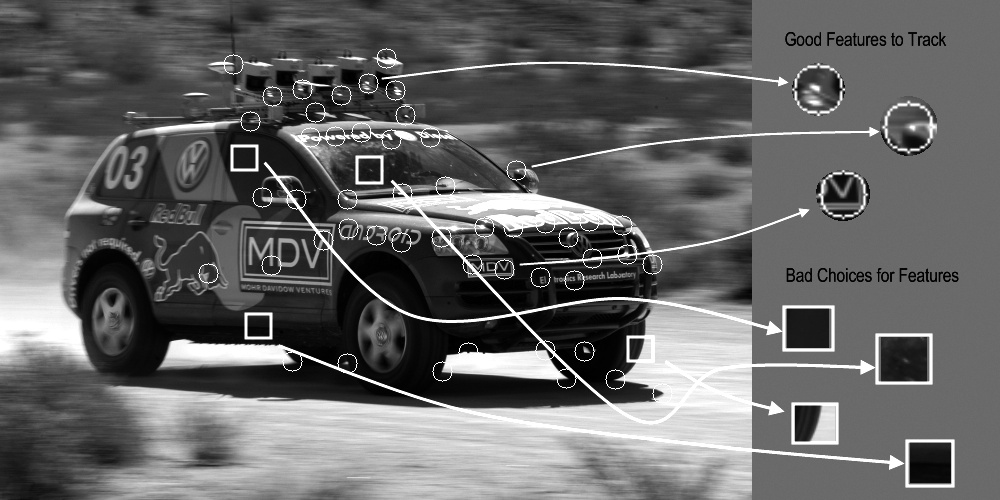
Figure 10-1. The points in circles are good points to track, whereas those in boxes—even sharply defined edges—are poor choices
Returning to our intuition from the large blank wall, we might be tempted to look for points that have some significant change in them—for example, a strong derivative. It turns out that this is not enough, but it's a start. A point to which a strong derivative is associated may be on an edge of some kind, but it could look like all of the other points along the same edge (see the aperture problem diagrammed in Figure 10-8 and discussed in the section titled "Lucas-Kanade Technique").
However, if strong derivatives are observed in two orthogonal directions then we can hope that this point is more likely to be unique. For this reason, many trackable features are called corners. Intuitively, corners—not edges—are the points that contain enough information to be picked out from one frame to the next.
The most commonly used definition of a corner was provided by Harris [Harris88]. This definition relies on the matrix of the second-order derivatives
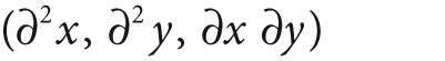
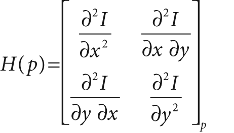
of the image intensities. We can think of the second-order derivatives of images, taken at all points in the image, as forming new "second-derivative images" or, when combined together, a new Hessian image. This terminology comes from the Hessian matrix around a point, which is defined in two dimensions by:
For the Harris corner, we consider the autocorrelation matrix of the second derivative images over a small window around each point. Such a matrix is defined as follows:
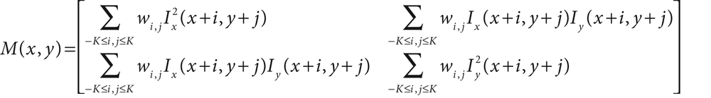
(Here wi,j is a weighting term that can be uniform but is often used to create an effectively non-square window, by setting some entries to zero, or Gaussian or other weighting) Corners, by Harris's definition, are places in the image where the autocorrelation matrix of the second derivatives has two large eigenvalues. In essence this means that there is texture (or edges) going in at least two separate directions centered around such a point, just as real corners have at least two edges meeting in a point. Second derivatives are useful because they do not respond to uniform gradients.[143] This definition has the further advantage that, when we consider only the eigenvalues of the autocorrelation matrix, we are considering quantities that are invariant also to rotation, which is important because objects that we are tracking might rotate as well as move. Observe also that these two eigenvalues do more than determine if a point is a good feature to track; they also provide an identifying signature for the point.
Harris's original definition involved taking the determinant of H(p), subtracting the trace of H(p) (with some weighting coefficient), and then comparing this difference to a predetermined threshold. It was later found by Shi and Tomasi [Shi94] that good corners resulted as long as the smaller of the two eigenvalues was greater than a minimum threshold. Shi and Tomasi's method was not only sufficient but in many cases gave more satisfactory results than Harris's method.
The cvGoodFeaturesToTrack() routine implements the
Shi and Tomasi definition. This function conveniently computes the second derivatives (using
the Sobel operators) that are needed and from those computes the needed eigenvalues.
It then returns a list of the points that meet our definition of being good for
tracking.
void cvGoodFeaturesToTrack(
    const CvArr*   image,
    CvArr*         eigImage,
    CvArr*         tempImage,
    CvPoint2D32f*  corners,
    int*           corner_count,
    double         quality_level,
    double         min_distance,
    const CvArr*   mask          = NULL,
    int            block_size    = 3,
    int            use_harris    = 0,
    double         k             = 0.4
);
In this case, the input image should be an 8-bit or
32-bit (i.e., IPL_DEPTH_8U or IPL_DEPTH_32F) single-channel image. The next two arguments are single-channel
32-bit images of the same size. Both tempImage and
eigImage are used as scratch by the algorithm, but the
resulting contents of eigImage are meaningful. In
particular, each entry there contains the minimal eigenvalue for the corresponding point in
the input image. Here corners is an array of 32-bit
points (CvPoint2D32f) that contain the result points
after the algorithm has run; you must allocate this array before calling cvGoodFeatures ToTrack(). Naturally, since you allocated that
array, you only allocated a finite amount of memory. The corner_count indicates the maximum number of points for which there is space to
return. After the routine exits, corner_count is
overwritten by the number of points that were actually found. The parameter quality_level indicates the minimal acceptable lower eigenvalue
for a point to be included as a corner. The actual minimal eigenvalue used for the cutoff is
the product of the quality_level and the largest lower
eigenvalue observed in the image. Hence, the quality_level should not exceed 1 (a typical value might be 0.10 or 0.01). Once
these candidates are selected, a further culling is applied so that multiple points within a
small region need not be included in the response. In particular, the min_distance guarantees that no two returned points are within
the indicated number of pixels.
The optional mask is the usual image, interpreted as
Boolean values, indicating which points should and which points should not be considered as
possible corners. If set to NULL, no mask is used. The
block_size is the region around a given pixel that is
considered when computing the autocorrelation matrix of derivatives. It turns out that it is
better to sum these derivatives over a small window than to compute their value at only a
single point (i.e., at a block_size of 1). If use_harris is nonzero, then the Harris corner definition is used
rather than the Shi-Tomasi definition. If you set use_harris to a nonzero value, then the value k is the weighting coefficient used to set the relative weight given to the
trace of the autocorrelation matrix Hessian compared to the determinant of the same
matrix.
Once you have called cvGoodFeaturesToTrack(), the
result is an array of pixel locations that you hope to find in another similar image. For
our current context, we are interested in looking for these features in subsequent frames of
video, but there are many other applications as well. A similar technique can be used when
attempting to relate multiple images taken from slightly different viewpoints. We will
re-encounter this issue when we discuss stereo vision in later chapters.
[143] A gradient is derived from first derivatives. If first derivatives are uniform (constant), then second derivatives are 0.