Subpixel Corners

If you are processing images for the purpose of extracting geometric measurements, as opposed to extracting features for recognition, then you will normally need more resolution than the simple pixel values supplied by cvGoodFeaturesToTrack(). Another way of saying this is that such pixels come with integer coordinates whereas we sometimes require real-valued coordinates—for example, pixel (8.25, 117.16).

One might imagine needing to look for a sharp peak in image values, only to be frustrated by the fact that the peak's location will almost never be in the exact center of a camera pixel element. To overcome this, you might fit a curve (say, a parabola) to the image values and then use a little math to find where the peak occurred between the pixels. Subpixel detection techniques are all about tricks like this (for a review and newer techniques, see Lucchese [Lucchese02] and Chen [Chen05]). Common uses of image measurements are tracking for three-dimensional reconstruction, calibrating a camera, warping partially overlapping views of a scene to stitch them together in the most natural way, and finding an external signal such as precise location of a building in a satellite image.

Subpixel corner locations are a common measurement used in camera calibration or when tracking to reconstruct the camera's path or the three-dimensional structure of a tracked object. Now that we know how to find corner locations on the integer grid of pixels, here's the trick for refining those locations to subpixel accuracy: We use the mathematical fact that the dot product between a vector and an orthogonal vector is 0; this situation occurs at corner locations, as shown in Figure 10-2.

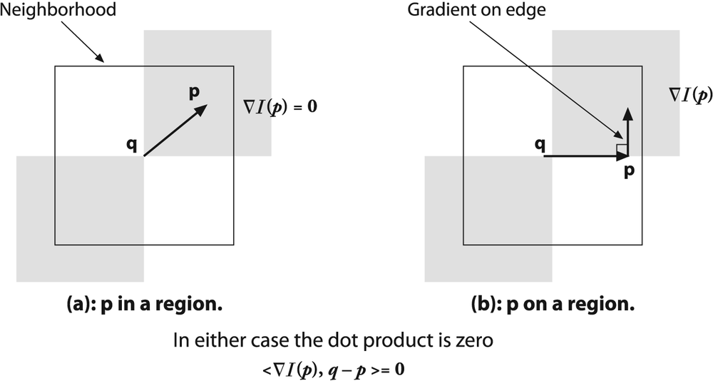
Figure 10-2. Finding corners to subpixel accuracy: (a) the image area around the point p is uniform and so its gradient is 0; (b) the gradient at the edge is orthogonal to the vector q-p along the edge; in either case, the dot product between the gradient at p and the vector q-p is 0 (see text)

In the figure, we assume a starting corner location q that is near the actual subpixel corner location. We examine vectors starting at point q and ending at p. When p is in a nearby uniform or "flat" region, the gradient there is 0. On the other hand, if the vector q-p aligns with an edge then the gradient at p on that edge is orthogonal to the vector q-p. In either case, the dot product between the gradient at p and the vector q-p is 0. We can assemble many such pairs of the gradient at a nearby point p and the associated vector q-p, set their dot product to 0, and solve this assemblage as a system of equations; the solution will yield a more accurate subpixel location for q, the exact location of the corner.

The function that does subpixel corner finding is cvFindCornerSubPix():

void cvFindCornerSubPix(
    const CvArr*    image,
    CvPoint2D32f*   corners,
    int             count,
    CvSize          win,
    CvSize          zero_zone,
    CvTermCriteria  criteria
);

The input image is a single-channel, 8-bit, grayscale image. The corners structure contains integer pixel locations, such as those obtained from routines like cvGoodFeatures ToTrack(), which are taken as the initial guesses for the corner locations; count holds how many points there are to compute.

The actual computation of the subpixel location uses a system of dot-product expressions that all equal 0 (see Figure 10-2), where each equation arises from considering a single pixel in the region around p. The parameter win specifies the size of window from which these equations will be generated. This window is centered on the original integer corner location and extends outward in each direction by the number of pixels specified in win (e.g., if win.width = 4 then the search area is actually 4 + 1 + 4 = 9 pixels wide). These equations form a linear system that can be solved by the inversion of a single autocorrelation matrix (not related to the autocorrelation matrix encountered in our previous discussion of Harris corners). In practice, this matrix is not always invertible owing to small eigenvalues arising from the pixels very close to p. To protect against this, it is common to simply reject from consideration those pixels in the immediate neighborhood of p. The parameter zero_zone defines a window (analogously to win, but always with a smaller extent) that will not be considered in the system of constraining equations and thus the autocorrelation matrix. If no such zero zone is desired then this parameter should be set to cvSize(-1,-1).

Once a new location is found for q, the algorithm will iterate using that value as a starting point and will continue until the user-specified termination criterion is reached. Recall that this criterion can be of type CV_TERMCRIT_ITER or of type CV_TERMCRIT_EPS (or both) and is usually constructed with the cvTermCriteria() function. Using CV_TERMCRIT_EPS will effectively indicate the accuracy you require of the subpixel values. Thus, if you specify 0.10 then you are asking for subpixel accuracy down to one tenth of a pixel.