In this section we will look at two techniques, mean-shift and camshift (where "camshift" stands for "continuously adaptive mean-shift"). The former is a general technique for data analysis (discussed in Chapter 9 in the context of segmentation) in many applications, of which computer vision is only one. After introducing the general theory of mean-shift, we'll describe how OpenCV allows you to apply it to tracking in images. The latter technique, camshift, builds on mean-shift to allow for the tracking of objects whose size may change during a video sequence.
The mean-shift algorithm [149] is a robust method of finding local extrema in the density distribution of a data set. This is an easy process for continuous distributions; in that context, it is essentially just hill climbing applied to a density histogram of the data. [150] For discrete data sets, however, this is a somewhat less trivial problem.
The descriptor "robust" is used here in its formal statistical sense; that is, mean-shift ignores outliers in the data. This means that it ignores data points that are far away from peaks in the data. It does so by processing only those points within a local window of the data and then moving that window.
The mean-shift algorithm runs as follows.
Choose a search window:
its initial location;
its type (uniform, polynomial, exponential, or Gaussian);
its shape (symmetric or skewed, possibly rotated, rounded or rectangular);
its size (extent at which it rolls off or is cut off).
Compute the window's (possibly weighted) center of mass.
Center the window at the center of mass.
Return to step 2 until the window stops moving (it always will). [151]
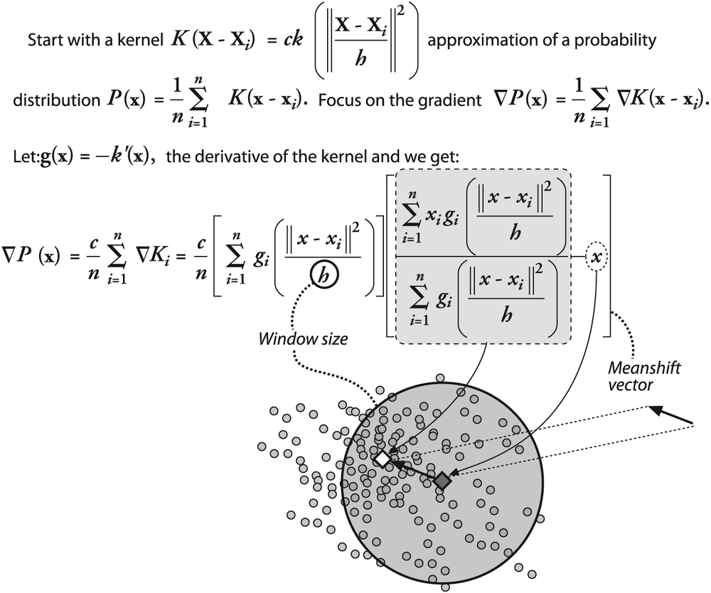
To give a little more formal sense of what the mean-shift algorithm is: it is related to the discipline of kernel density estimation, where by "kernel" we refer to a function that has mostly local focus (e.g., a Gaussian distribution). With enough appropriately weighted and sized kernels located at enough points, one can express a distribution of data entirely in terms of those kernels. Mean-shift diverges from kernel density estimation in that it seeks only to estimate the gradient (direction of change) of the data distribution. When this change is 0, we are at a stable (though perhaps local) peak of the distribution. There might be other peaks nearby or at other scales.
Figure 10-11 shows the equations involved in the mean-shift algorithm. These equations can be simplified by considering a rectangular kernel, [152] which reduces the mean-shift vector equation to calculating the center of mass of the image pixel distribution:
Here the zeroth moment is calculated as:
and the first moments are:
The mean-shift vector in this case tells us to recenter the mean-shift window over the calculated center of mass within that window. This movement will, of course, change what is "under" the window and so we iterate this recentering process. Such recentering will always converge to a mean-shift vector of 0 (i.e., where no more centering movement is possible). The location of convergence is at a local maximum (peak) of the distribution under the window. Different window sizes will find different peaks because "peak" is fundamentally a scale-sensitive construct.
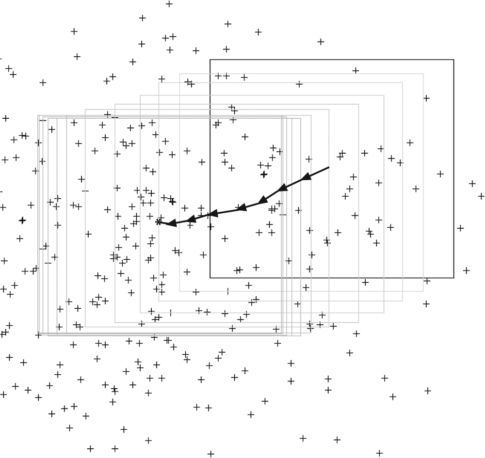
In Figure 10-12 we see an example of a two-dimensional distribution of data and an initial (in this case, rectangular) window. The arrows indicate the process of convergence on a local mode (peak) in the distribution. Observe that, as promised, this peak finder is statistically robust in the sense that points outside the mean-shift window do not affect convergence—the algorithm is not "distracted" by far-away points.
In 1998, it was realized that this mode-finding algorithm could be used to track moving objects in video [Bradski98a; Bradski98b], and the algorithm has since been greatly extended [Comaniciu03]. The OpenCV function that performs mean-shift is implemented in the context of image analysis. This means in particular that, rather than taking some arbitrary set of data points (possibly in some arbitrary number of dimensions), the OpenCV implementation of mean-shift expects as input an image representing the density distribution being analyzed. You could think of this image as a two-dimensional histogram measuring the density of points in some two-dimensional space. It turns out that, for vision, this is precisely what you want to do most of the time: it's how you can track the motion of a cluster of interesting features.
Figure 10-12. Mean-shift algorithm in action: an initial window is placed over a two-dimensional array of data points and is successively recentered over the mode (or local peak) of its data distribution until convergence
int cvMeanShift(
    const CvArr*      prob_image,
    CvRect            window,
    CvTermCriteria    criteria,
    CvConnectedComp*  comp
);
In cvMeanShift(), the prob_image, which represents the density of probable locations, may be only
one channel but of either type (byte or float). The window is set at the initial desired location and size of the kernel
window. The termination criteria has been described
elsewhere and consists mainly of a maximum limit on number of mean-shift movement
iterations and a minimal movement for which we consider the window locations to have
converged. [153] The connected component comp contains the
converged search window location in comp->rect,
and the sum of all pixels under the window is kept in the comp->area field.
The function cvMeanShift() is one expression of
the mean-shift algorithm for rectangular windows, but it may also be used for tracking.
In this case, you first choose the feature distribution to represent an object (e.g.,
color + texture), then start the mean-shift window over the feature distribution
generated by the object, and finally compute the chosen feature distribution over the
next video frame. Starting from the current window location, the mean-shift algorithm
will find the new peak or mode of the feature distribution, which (presumably) is
centered over the object that produced the color and texture in the first place. In this
way, the mean-shift window tracks the movement of the object frame by frame.
A related algorithm is the Camshift tracker. It differs from the meanshift in that the search window adjusts itself in size. If you have well-segmented distributions (say face features that stay compact), then this algorithm will automatically adjust itself for the size of face as the person moves closer to and further from the camera. The form of the Camshift algorithm is:
int cvCamShift(
    const CvArr*     prob_image,
    CvRect           window,
    CvTermCriteria   criteria,
    CvConnectedComp* comp,
    CvBox2D*         box         = NULL
);
The first four parameters are the same as for the cvMeanShift() algorithm. The box
parameter, if present, will contain the newly resized box, which also includes the
orientation of the object as computed via second-order moments. For tracking applications,
we would use the resulting resized box found on the
previous frame as the window in the next frame.
[149] Because mean-shift is a fairly deep topic, our discussion here is aimed mainly at developing intuition for the user. For the original formal derivation, see Fukunaga [Fukunaga90] and Comaniciu and Meer [Comaniciu99].
[150] The word "essentially" is used because there is also a scale-dependent aspect of mean-shift. To be exact: mean-shift is equivalent in a continuous distribution to first convolving with the mean-shift kernel and then applying a hill-climbing algorithm.
[151] Iterations are typically restricted to some maximum number or to some epsilon change in center shift between iterations; however, they are guaranteed to converge eventually.
[152] A rectangular kernel is a kernel with no falloff with distance from the center, until a single sharp transition to zero value. This is in contrast to the exponential falloff of a Gaussian kernel and the falloff with the square of distance from the center in the commonly used Epanechnikov kernel.
[153] Again, mean-shift will always converge, but convergence may be very slow near the local peak of a distribution if that distribution is fairly "flat" there.


