A final topic of interest in this chapter is that of general line fitting. This can
arise for many reasons and in a many contexts. We have chosen to discuss it here because one
especially frequent context in which line fitting arises is that of analyzing points in
three dimensions (although the function described here can also fit lines in two
dimensions). Line-fitting algorithms generally use statistically robust techniques [Inui03,
Meer91, Rousseeuw87]. The OpenCV line-fitting algorithm cvFitLine() can be used whenever line fitting is needed.
void cvFitLine(
  const CvArr* points,
  int          dist_type,
  double       param,
  double       reps,
  double       aeps,
  float*       line
);
The array points can be an
N-by-2 or N-by-3 matrix of floating-point values
(accommodating points in two or three dimensions), or it can be a sequence of cvPointXXX structures. [226] The argument dist_type indicates the distance
metric that is to be minimized across all of the points (see Table 12-3).
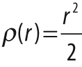
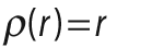
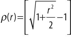
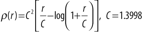
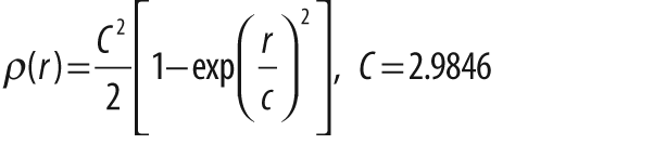

The parameter param is used to set the parameter C
listed in Table 12-3. This can be left set
to 0, in which case the listed value from the table will be selected. We'll get back to
reps and aeps after
describing line.
The argument line is the location at which the result
is stored. If points is an N-by-2
array, then line should be a pointer to an array of four
floating-point numbers (e.g., float array[4]). If
points is an N-by-3 array, then
line should be a pointer to an array of six
floating-point numbers (e.g., float array[6]). In the
former case, the return values will be (vx,
vy, x0,
y0), where (vx,
vy) is a normalized vector parallel to the fitted line
and (x0, y0) is a point
on that line. Similarly, in the latter (three-dimensional) case, the return values will be
(vx, vy,
vz, x0, y0,
z0), where (vx,
vy, vz) is a normalized vector
parallel to the fitted line and (x0,
y0,
z0) is a point on that line. Given this line
representation, the estimation accuracy parameters reps
and aeps are as follows: reps is the requested accuracy of x0, y0[,
z0] estimates and aeps is the requested
angular accuracy for vx, vy[, vz]. The OpenCV
documentation recommends values of 0.01 for both accuracy values.
cvFitLine() can fit lines in two or three dimensions.
Since line fitting in two dimensions is commonly needed and since three-dimensional
techniques are of growing importance in OpenCV (see Chapter 14), we
will end with a program for line fitting, shown in Example 12-4. [227] In this code we first synthesize some 2D points noisily around a line, then add
some random points that have nothing to do with the line (called
outlier points), and finally fit a line to the points and display it.
The cvFitLine() routine is good at ignoring the outlier
points; this is important in real applications, where some measurements might be corrupted
by high noise, sensor failure, and so on.
Example 12-4. Two-dimensional line fitting
#include "cv.h"
#include "highgui.h"
#include <math.h>

int main( int argc, char** argv )
{
  IplImage* img = cvCreateImage( cvSize( 500, 500 ), 8, 3 );
  CvRNG rng = cvRNG(-1);

  cvNamedWindow( "fitline", 1 );

  for(;;) {

  char key;
  int i;
  int count    = cvRandInt(&rng)%100 + 1;
  int outliers = count/5;
  float a      = cvRandReal(&rng)*200;
  float b      = cvRandReal(&rng)*40;
  float angle  = cvRandReal(&rng)*CV_PI;
  float cos_a  = cos(angle);
  float sin_a  = sin(angle);
  CvPoint pt1, pt2;
  CvPoint* points = (CvPoint*)malloc( count * sizeof(points[0]));
  CvMat pointMat = cvMat( 1, count, CV_32SC2, points );
  float line[4];
  float d, t;

  b = MIN(a*0.3, b);
  // generate some points that are close to the line
  //
  for( i = 0; i < count - outliers; i++ ) {
      float x = (cvRandReal(&rng)*2-1)*a;
      float y = (cvRandReal(&rng)*2-1)*b;
      points[i].x = cvRound(x*cos_a - y*sin_a + img->width/2);
      points[i].y = cvRound(x*sin_a + y*cos_a + img->height/2);
  }

  // generate "completely off" points
  //
  for( ; i < count; i++ ) {
      points[i].x = cvRandInt(&rng) % img->width;
      points[i].y = cvRandInt(&rng) % img->height;
  }

  // find the optimal line
  //
  cvFitLine( &pointMat, CV_DIST_L1, 1, 0.001, 0.001, line );
  cvZero( img );

  // draw the points
  //
  for( i = 0; i < count; i++ )
    cvCircle(
      img,
      points[i],
      2,
     (i < count - outliers) ? CV_RGB(255, 0, 0) : CV_RGB(255,255,0),
     CV_FILLED, CV_AA,
     0
    );
  // ... and the line long enough to cross the whole image
  d = sqrt((double)line[0]*line[0] + (double)line[1]*line[1]);
  line[0] /= d;
  line[1] /= d;
  t = (float)(img->width + img->height);
  pt1.x = cvRound(line[2] - line[0]*t);
  pt1.y = cvRound(line[3] - line[1]*t);
  pt2.x = cvRound(line[2] + line[0]*t);
  pt2.y = cvRound(line[3] + line[1]*t);
  cvLine( img, pt1, pt2, CV_RGB(0,255,0), 3, CV_AA, 0 );

  cvShowImage( "fitline", img );

  key = (char) cvWaitKey(0);
  if( key == 27 || key == 'q' || key == 'Q' ) // 'ESC'
      break;
  free( points );
 }
 cvDestroyWindow( "fitline" );
 return 0;
}