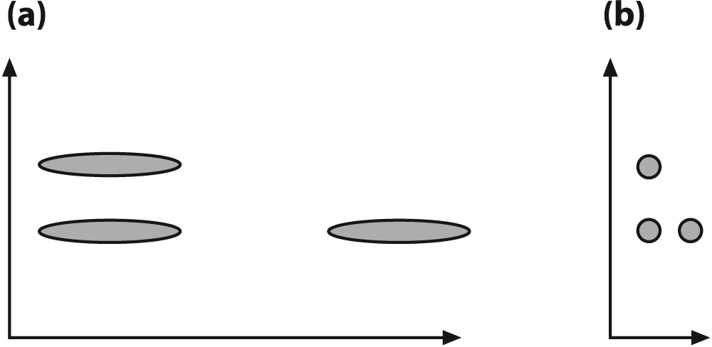
The Mahalanobis distance is a distance measure that accounts for the covariance or "stretch" of the space in which the data lies. If you know what a Z-score is then you can think of the Mahalanobis distance as a multidimensional analogue of the Z-score. Figure 13-4(a) shows an initial distribution between three sets of data that make the vertical sets look closer together. When we normalize the space by the covariance in the data, we see in Figure 13-4(b) that that horizontal data sets are actually closer together. This sort of thing occurs frequently; for instance, if we are comparing people's height in meters with their age in days, we'd see very little variance in height to relate to the large variance in age. By normalizing for the variance we can obtain a more realistic comparison of variables. Some classifiers such as K-nearest neighbors deal poorly with large differences in variance, whereas other algorithms (such as decision trees) don't mind it.
We can already get a hint for what the Mahalanobis distance must be by looking at Figure 13-4;[239] we must somehow divide out the covariance of the data while measuring distance. First, let us review what covariance is. Given a list X of N data points, where each data point may be of dimension (vector length) K with mean vector μx (consisting of individual means μ1,…,K), the covariance is a K-by-K matrix given by:
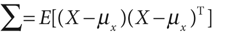
where E[·] is the expectation operator. OpenCV makes computing the covariance matrix easy, using
void cvCalcCovarMatrix(
  const CvArr** vects,
  int           count,
  CvArr*        cov_mat,
  CvArr*        avg,
  int           flags
);
This function is a little bit tricky. Note that vects
is a pointer to a pointer of CvArr. This implies that we
have vects[0] through vects[count-1], but it actually depends on the flags settings as described in what follows. Basically, there are two
cases.
Vectsis a 1D vector of pointers to 1D vectors or 2D matrices (the two dimensions are to accommodate images). That is, eachvects[i]can point to a 1D or a 2D vector, which occurs if neitherCV_COV_ROWSnorCV_COV_COLSis set. The accumulating covariance computation is scaled or divided by the number of data points given bycountifCV_COVAR_SCALEis set.Often there is only one input vector, so use only
vects[0]if eitherCV_COVAR_ROWSorCV_COVAR_COLSis set. If this is set, then scaling by the value given bycountis ignored in favor of the number of actual data vectors contained invects[0]. All the data points are then in:Figure 13-4. The Mahalanobis computation allows us to reinterpret the data's covariance as a "stretch" of the space: (a) the vertical distance between raw data sets is less than the horizontal distance; (b) after the space is normalized for variance, the horizontal distance between data sets is less than the vertical distance
Vects can be of types 8UC1,
16UC1, 32FC1, or 64FC1. In any case, vects contains a list of K-dimensional data
points. To reiterate: count is how many vectors there are
in vects[] for case 1 (CV_COVAR_ROWS and CV_COVAR_COLS not set);
for case 2a and 2b (CV_COVAR_ROWS or CV_COVAR_COLS is set), count
is ignored and the actual number of vectors in vects[0]
is used instead. The resulting K-by-K covariance
matrix will be returned in cov_mat, and it can be of type
CV_32FC1 or CV_64FC1. Whether or not the vector avg is
used depends on the settings of flags (see listing that
follows). If avg is used then it has the same type as
vects and contains the K-feature
averages across vects. The parameter flags can have many combinations of settings formed by adding
values together (for more complicated applications, refer to the …/opencv/docs/ref/opencvref_cxcore.htm documentation). In general, you will
set flags to one of the following.
-
CV_COVAR_NORMAL Do the regular type of covariance calculation as in the previously displayed equation. Average the results by the number in
countifCV_COVAR_SCALEis not set; otherwise, average by the number of data points invects[0].-
CV_COVAR_SCALE Normalize the computed covariance matrix.
-
CV_COVAR_USE_AVG Use the
avgmatrix instead of automatically calculating the average of each feature. Setting this saves on computation time if you already have the averages (e.g., by having calledcvAvg()yourself); otherwise, the routine will compute these averages for you.[240]
Most often you will combine your data into one big matrix, let's say by rows of data
points; then flags would be set as flags = CV_COVAR_NORMAL |
CV_COVAR_SCALE | CV_COVAR_ROWS.
We now have the covariance matrix. For Mahalanobis distance, however, we'll need to divide out the variance of the space and so will need the inverse covariance matrix. This is easily done by using:
double cvInvert(
  const CvArr* src,
  CvArr*       dst,
  int          method = CV_LU
);
In cvInvert(), the src matrix should be the covariance matrix calculated before and dst should be a same sized matrix, which will be filled with the
inverse on return. You could leave the method at its
default value, CV_LU, but it is better to set the method
to CV_SVD_SYM.[241]
With the inverse covariance matrix

finally in hand, we can move on to the Mahalanobis distance measure. This measure is much like the Euclidean distance measure, which is the square root of the sum of squared differences between two vectors x and y, but it divides out the covariance of the space:
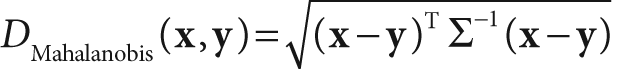
This distance is just a number. Note that if the covariance matrix is the identity
matrix then the Mahalanobis distance is equal to the Euclidean distance. We finally arrive
at the actual function that computes the Mahalanobis distance. It takes two input vectors
(vec1 and vec2) and
the inverse covariance in mat, and it returns the
distance as a double:
double cvMahalanobis(
  const CvArr* vec1,
  const CvArr* vec2,
  CvArr*       mat
);
The Mahalanobis distance is an important measure of similarity between two different data points in a multidimensional space, but is not a clustering algorithm or classifier itself. Let us now move on, starting with the most frequently used clustering algorithm: K-means.
[239] Note that Figure 13-4 has a diagonal covariance matrix, which entails independent X and Y variance rather than actual covariance. This was done to make the explanation simple. In reality, data is often "stretched" in much more interesting ways.
[240] A precomputed average data vector should be passed if the user has a more statistically justified value of the average or if the covariance matrix is computed by blocks.
[241] CV_SVD could also be used in this case, but it is
somewhat slower and less accurate than CV_SVD_SYM.
CV_SVD_SYM, even if it is slower than CV_LU, still should be used if the dimensionality of the space is much
smaller than the number of data points. In such a case the overall computing time will
be dominated by cvCalcCovarMatrix() anyway. So it may
be wise to spend a little bit more time on computing inverse covariance matrix more
accurately (much more accurately, if the set of points is concentrated in a subspace of
a smaller dimensionality). Thus, CV_SVD_SYM is
usually the best choice for this task.