We now turn to the final tree-based technique in OpenCV: the Haar classifier, which builds a boosted rejection cascade. It has a different format from the rest of the ML library in OpenCV because it was developed earlier as a full-fledged face-recognition application. Thus, we cover it in detail and show how it can be trained to recognize faces and other rigid objects.
Computer vision is a broad and fast-changing field, so the parts of OpenCV that implement a specific technique—rather than a component algorithmic piece—are more at risk of becoming out of date. The face detector that comes with OpenCV is in this "risk" category. However, face detection is such a common need that it is worth having a baseline technique that works fairly well; also, the technique is built on the well-known and often used field of statistical boosting and thus is of more general use as well. In fact, several companies have engineered the "face" detector in OpenCV to detect "mostly rigid" objects (faces, cars, bikes, human body) by training new detectors on many thousands of selected training images for each view of the object. This technique has been used to create state-of-the-art detectors, although with a different detector trained for each view or pose of the object. Thus, the Haar classifier is a valuable tool to keep in mind for such recognition tasks.
OpenCV implements a version of the face-detection technique first developed by Paul
Viola and Michael Jones—commonly known as the Viola-Jones detector[261]—and later extended by Rainer Lienhart and Jochen Maydt[262] to use diagonal features (more on this distinction to
follow). OpenCV refers to this detector as the "Haar classifier" because it uses Haar features[263] or, more precisely, Haar-like wavelets that consist of adding and subtracting
rectangular image regions before thresholding the result. OpenCV ships with a set of
pretrained object-recognition files, but the code also allows you to train and store new
object models for the detector. We note once again that the training (createsamples(), haartraining()) and detecting (cvHaarDetectObjects()) code works well on any objects (not just
faces) that are consistently textured and mostly rigid.
The pretrained objects that come with OpenCV for this detector are in …/opencv/data/haarcascades, where the model that works best for frontal face detection is haarcascade_frontalface_alt2.xml. Side face views are harder to detect accurately with this technique (as we shall describe shortly), and those shipped models work less well. If you end up training good object models, perhaps you will consider contributing them as open source back to the community.
The Haar classifier that is included in OpenCV is a supervised classifier (these were discussed at the beginning of the chapter). In this case we typically present histogram- and size-equalized image patches to the classifier, which are then labeled as containing (or not containing) the object of interest, which for this classifier is most commonly a face.
The Viola-Jones detector uses a form of AdaBoost but organizes it as a rejection cascade of nodes, where each node is a multitree AdaBoosted classifier designed to have high (say, 99.9%) detection rate (low false negatives, or missed faces) at the cost of a low (near 50%) rejection rate (high false positives, or "nonfaces" wrongly classified). For each node, a "not in class" result at any stage of the cascade terminates the computation, and the algorithm then declares that no face exists at that location. Thus, true class detection is declared only if the computation makes it through the entire cascade. For instances where the true class is rare (e.g., a face in a picture), rejection cascades can greatly reduce total computation because most of the regions being searched for a face terminate quickly in a nonclass decision.
Boosted classifiers were discussed earlier in this chapter. For the Viola-Jones rejection cascade, the weak classifiers that it boosts in each node are decision trees that often are only one level deep (i.e., "decision stumps"). A decision stump is allowed just one decision of the following form: "Is the value v of a particular feature f above or below some threshold t"; then, for example, a "yes" indicates face and a "no" indicates no face:
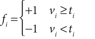
The number of Haar-like features that the Viola-Jones classifier uses in each weak classifier can be set in training, but mostly we use a single feature (i.e., a tree with a single split) or at most about three features. Boosting then iteratively builds up a classifier as a weighted sum of these kinds of weak classifiers. The Viola-Jones classifier uses the classification function:

Here, the sign function returns –1 if the number is less than 0, 0 if the number equals 0, and +1 if the number is positive. On the first pass through the data set, we learn the threshold tl of f1 that best classifies the input. Boosting then uses the resulting errors to calculate the weighted vote w1. As in traditional AdaBoost, each feature vector (data point) is also reweighted low or high according to whether it was classified correctly or not[264] in that iteration of the classifier. Once a node is learned this way, the surviving data from higher up in the cascade is used to train the next node and so on.
The Viola-Jones classifier employs AdaBoost at each node in the cascade to learn a high detection rate at the cost of low rejection rate multitree (mostly multistump) classifier at each node of the cascade. This algorithm incorporates several innovative features.
It uses Haar-like input features: a threshold applied to sums and differences of rectangular image regions.
Its integral image technique enables rapid computation of the value of rectangular regions or such regions rotated 45 degrees (see Chapter 6). This data structure is used to accelerate computation of the Haar-like input features.
It uses statistical boosting to create binary (face–not face) classification nodes characterized by high detection and weak rejection.
It organizes the weak classifier nodes of a rejection cascade. In other words: the first group of classifiers is selected that best detects image regions containing an object while allowing many mistaken detections; the next classifier group[265] is the second-best at detection with weak rejection; and so forth. In test mode, an object is detected only if it makes it through the entire cascade.[266]
The Haar-like features used by the classifier are shown in Figure 13-14. At all scales, these features form the "raw material" that will be used by the boosted classifiers. They are rapidly computed from the integral image (see Chapter 6) representing the original grayscale image.

Figure 13-14. Haar-like features from the OpenCV source distribution (the rectangular and rotated regions are easily calculated from the integral image): in this diagrammatic representation of the wavelets, the light region is interpreted as "add that area" and the dark region as "subtract that area"
Viola and Jones organized each boosted classifier group into nodes of a rejection cascade, as shown in Figure 13-15. In the figure, each of the nodes Fj contains an entire boosted cascade of groups of decision stumps (or trees) trained on the Haar-like features from faces and nonfaces (or other objects the user has chosen to train on). Typically, the nodes are ordered from least to most complex so that computations are minimized (simple nodes are tried first) when rejecting easy regions of the image. Typically, the boosting in each node is tuned to have a very high detection rate (at the usual cost of many false positives). When training on faces, for example, almost all (99.9%) of the faces are found but many (about 50%) of the nonfaces are erroneously "detected" at each node. But this is OK because using (say) 20 nodes will still yield a face detection rate (through the whole cascade) of 0.99920 ≈ 98% with a false positive rate of only 0.520 ≈ 0.0001%!
During the run mode, a search region of different sizes is swept over the original image. In practice, 70–80% of nonfaces are rejected in the first two nodes of the rejection cascade, where each node uses about ten decision stumps. This quick and early "attentional reject" vastly speeds up face detection.
This technique implements face detection but is not limited to faces; it also works fairly well on other (mostly rigid) objects that have distinguishing views. That is, front views of faces work well; backs, sides, or fronts of cars work well; but side views of faces or "corner" views of cars work less well—mainly because these views introduce variations in the template that the "blocky" features (see next paragraph) used in this detector cannot handle well. For example, a side view of a face must catch part of the changing background in its learned model in order to include the profile curve. To detect side views of faces, you may try haarcascade_profileface.xml, but to do a better job you should really collect much more data than this model was trained with and perhaps expand the data with different backgrounds behind the face profiles. Again, profile views are hard for this classifier because it uses block features and so is forced to attempt to learn the background variability that "peaks" through the informative profile edge of the side view of faces. In training, it's more efficient to learn only (say) right profile views. Then the test procedure would be to (1) run the right-profile detector and then (2) flip the image on its vertical axis and run the right-profile detector again to detect left-facing profiles.
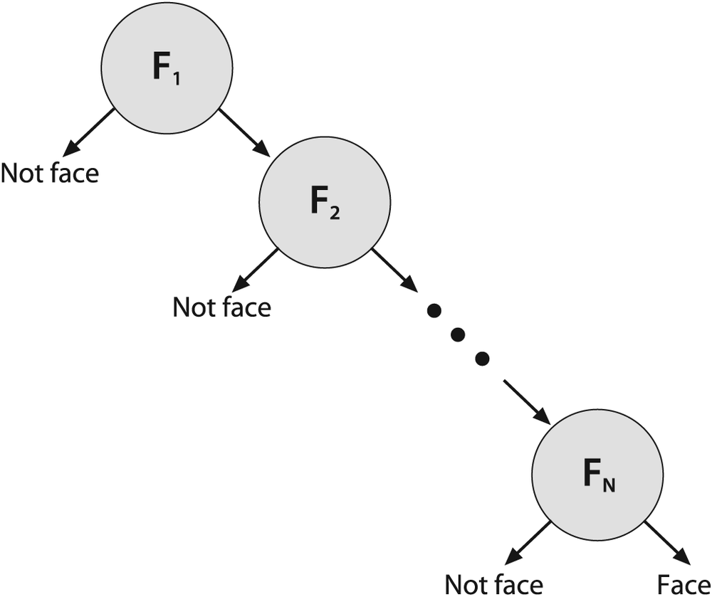
Figure 13-15. Rejection cascade used in the Viola-Jones classifier: each node represents a multitree boosted classifier ensemble tuned to rarely miss a true face while rejecting a possibly small fraction of nonfaces; however, almost all nonfaces have been rejected by the last node, leaving only true faces
As we have discussed, detectors based on these Haar-like features work well with "blocky" features—such as eyes, mouth, and hairline—but work less well with tree branches, for example, or when the object's outline shape is its most distinguishing characteristic (as with a coffee mug).
All that being said, if you are willing to gather lots of good, well-segmented data on fairly rigid objects, then this classifier can still compete with the best, and its construction as a rejection cascade makes it very fast to run (though not to train, however). Here "lots of data" means thousands of object examples and tens of thousands of nonobject examples. By "good" data we mean that one shouldn't mix, for instance, tilted faces with upright faces; instead, keep the data divided and use two classifiers, one for tilted and one for upright. "Well-segmented" data means data that is consistently boxed. Sloppiness in box boundaries of the training data will often lead the classifier to correct for fictitious variability in the data. For example, different placement of the eye locations in the face data location boxes can lead the classifier to assume that eye locations are not a geometrically fixed feature of the face and so can move around. Performance is almost always worse when a classifier attempts to adjust to things that aren't actually in the real data.
The detect_and_draw() code shown in Example 13-4 will detect faces and draw their found
locations in different-colored rectangles on the image. As shown in the fourth through
seventh (comment) lines, this code presumes that a previously trained classifier cascade
has been loaded and that memory for detected faces has been created.
Example 13-4. Code for detecting and drawing faces
// Detect and draw detected object boxes on image
// Presumes 2 Globals:
//  Cascade is loaded by:
//     cascade = (CvHaarClassifierCascade*)cvLoad( cascade_name,
//   0, 0, 0 );
//  AND that storage is allocated:
//  CvMemStorage* storage = cvCreateMemStorage(0);
//
void detect_and_draw(
  IplImage* img,
  double scale = 1.3
){
 static CvScalar colors[] = {
   {{0,0,255}}, {{0,128,255}},{{0,255,255}},{{0,255,0}},
   {{255,128,0}},{{255,255,0}},{{255,0,0}}, {{255,0,255}}
 }; //Just some pretty colors to draw with

 // IMAGE PREPARATION:
 //
 IplImage* gray = cvCreateImage( cvSize(img->width,img->height), 8, 1 );
 IplImage* small_img = cvCreateImage(
   cvSize( cvRound(img->width/scale), cvRound(img->height/scale)), 8, 1
 );
 cvCvtColor( img, gray, CV_BGR2GRAY );
 cvResize( gray, small_img, CV_INTER_LINEAR );
 cvEqualizeHist( small_img, small_img );

 // DETECT OBJECTS IF ANY
 //
 cvClearMemStorage( storage );
 CvSeq* objects = cvHaarDetectObjects(
   small_img,
   cascade,
   storage,
   1.1,
   2,
   0 /*CV_HAAR_DO_CANNY_PRUNING*/,
   cvSize(30, 30)
 );

 // LOOP THROUGH FOUND OBJECTS AND DRAW BOXES AROUND THEM
 //
 for(int i = 0; i < (objects ? objects->total : 0); i++ ) {
   CvRect* r = (CvRect*)cvGetSeqElem( objects, i );
   cvRectangle(
     img,
     cvPoint(r->x* scale, r->y* scale),
     cvPoint((r->x+r->width) *scale, (r->y+r->height) *scale)
     colors[i%8]
   )
 }
 cvReleaseImage( &graygray );
 cvReleaseImage( &small_img );
}
For convenience, in this code the detect_and_draw()
function has a static array of color vectors colors[]
that can be indexed to draw found faces in different colors. The classifier works on
grayscale images, so the color BGR image img passed
into the function is converted to grayscale using cvCvtColor() and then optionally resized in cvResize(). This is followed by histogram equalization via cvEqualizeHist(), which spreads out the brightness
values—necessary because the integral image features are based on differences of rectangle
regions and, if the histogram is not balanced, these differences might be skewed by
overall lighting or exposure of the test images. Since the classifier returns found object
rectangles as a sequence object CvSeq, we need to clear
the global storage that we're using for these returns by calling cvClearMemStorage(). The actual detection takes place just above the for{} loop, whose parameters are discussed in more detail
below. This loop steps through the found face rectangle regions and draws them in
different colors using cvRectangle(). Let us take a
closer look at detection function call:
CvSeq* cvHaarDetectObjects(
   const CvArr*             image,
   CvHaarClassifierCascade* cascade,
   CvMemStorage*            storage,
   double                   scale_factor  = 1.1,
   int                      min_neighbors = 3,
   int                      flags         = 0,
   CvSize                   min_size      = cvSize(0,0)
);
CvArr image is a grayscale image. If region of
interest (ROI) is set, then the function will respect that region. Thus, one way of
speeding up face detection is to trim down the image boundaries using ROI. The classifier
cascade is just the Haar feature cascade that we loaded with cvLoad() in the face detect code. The storage argument is an OpenCV "work buffer" for the algorithm; it is
allocated with cvCreateMemStorage(0) in the face
detection code and cleared for reuse with cvClearMemStorage(storage). The cvHaarDetectObjects() function scans the input image for faces at all scales.
Setting the scale_factor parameter determines how big
of a jump there is between each scale; setting this to a higher value means faster
computation time at the cost of possible missed detections if the scaling misses faces of
certain sizes. The min_neighbors parameter is a
control for preventing false detection. Actual face locations in an image tend to get
multiple "hits" in the same area because the surrounding pixels and scales often indicate
a face. Setting this to the default (3) in the face detection code indicates that we will
only decide a face is present in a location if there are at least three overlapping
detections. The flags parameter has four valid
settings, which (as usual) may be combined with the Boolean OR operator. The first is
CV_HAAR_DO_CANNY_PRUNING. Setting flags to this value causes flat regions (no lines) to be
skipped by the classifier. The second possible flag is CV_HAAR_SCALE_IMAGE, which tells the algorithm to scale the image rather than
the detector (this can yield some performance advantages in terms of how memory and cache
are used). The next flag option, CV_HAAR_FIND_BIGGEST_OBJECT, tells OpenCV to return only the largest object
found (hence the number of objects returned will be either one or none).[267] The final flag is CV_HAAR_DO_ROUGH_SEARCH,
which is used only with CV_HAAR_FIND_BIGGEST_OBJECT.
This flag is used to terminate the search at whatever scale the first candidate is found
(with enough neighbors to be considered a "hit"). The final parameter, min_size, is the smallest region in which to search for a
face. Setting this to a larger value will reduce computation at the cost of missing small
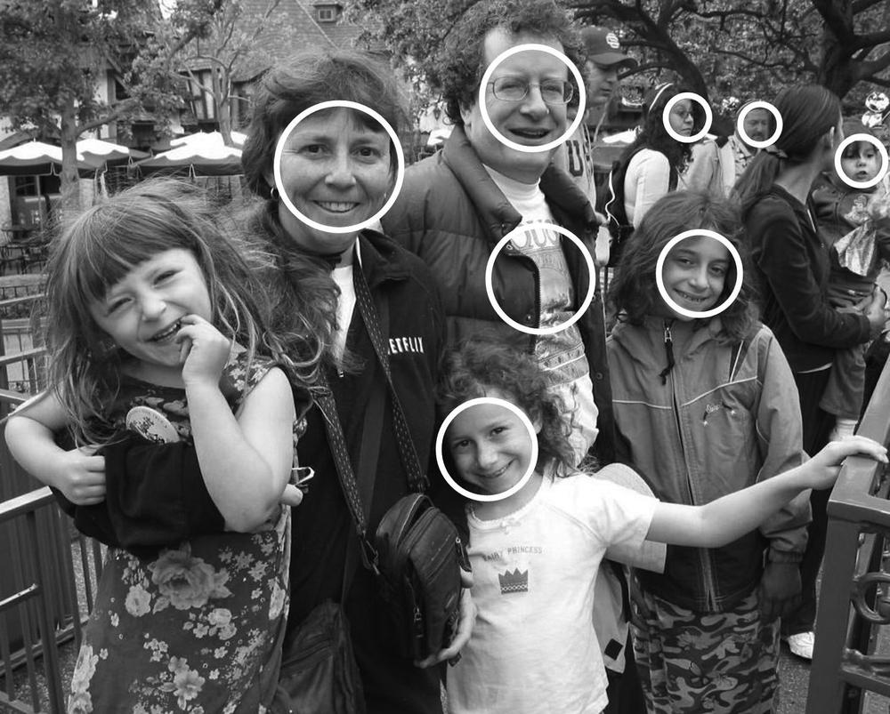
faces. Figure 13-16 shows results for using
the face-detection code on a scene with faces.
We've seen how to load and run a previously trained classifier cascade stored in an
XML file. We used the cvLoad() function to load it and
then used cvHaarDetectObjects() to find objects similar
to the ones it was trained on. We now turn to the question of how to train our own
classifiers to detect other objects such as eyes, walking people, cars, et cetera. We do this with the OpenCV haartraining application, which creates a classifier given a
training set of positive and negative samples. The four steps of training a classifier are
described next. (For more details, see the haartraining reference manual supplied with OpenCV in the opencv/apps/HaarTraining/doc directory.)
Gather a data set consisting of examples of the object you want to learn (e.g., front views of faces, side views of cars). These may be stored in one or more directories indexed by a text file in the following format:
<path>/img_name_1 count_1 x11 y11 w11 h11 x12 y12 . . .
<path>/img_name_2 count_2 x21 y21 w21 h21 x22 y22 . . .
 . . .
Each of these lines contains the path (if any) and file name of the image containing the object(s). This is followed by the count of how many objects are in that image and then a list of rectangles containing the objects. The format of the rectangles is the x- and y-coordinates of the upper left corner followed by the width and height in pixels.
Figure 13-16. Face detection on a park scene: some tilted faces are not detected, and there is also a false positive (shirt near the center); for the 1054-by-851 image shown, more than a million sites and scales were searched to achieve this result in about 1.5 seconds on a 2 GHz machine
To be more specific, if we had a data set of faces located in directory data/faces/, then the index file faces.idx might look like this:
data/faces/face_000.jpg 2 73 100 25 37 133 123 30 45
data/faces/face_001.jpg 1 155 200 55 78
 . . .
If you want your classifier to work well, you will need to gather a lot of high-quality data (1,000–10,000 positive examples). "High quality" means that you've removed all unnecessary variance from the data. For example, if you are learning faces, you should align the eyes (and preferably the nose and mouth) as much as possible. The intuition here is that otherwise you are teaching the classifier that eyes need not appear at fixed locations in the face but instead could be anywhere within some region. Since this is not true of real data, your classifier will not perform as well. One strategy is to first train a cascade on a subpart, say "eyes", which are easier to align. Then use eye detection to find the eyes and rotate/resize the face until the eyes are aligned. For asymmetric data, the "trick" of flipping an image on its vertical axis was described previously in the subsection "Works well on …".
Use the utility application
createsamplesto build a vector output file of the positive samples. Using this file, you can repeat the training procedure below on many runs, trying different parameters while using the same vector output file. For example:createsamples -vec faces.vec -info faces.idx -w 30 -h 40
This reads in the faces.idx file described in step 1 and outputs a formatted training file, faces.vec. Then
createsamplesextracts the positive samples from the images before normalizing and resizing them to the specified width and height (here, 30-by-40). Note thatcreatesamplescan also be used to synthesize data by applying geometric transformations, adding noise, altering colors, and so on. This procedure could be used (say) to learn a corporate logo, where you take just one image and put it through various distortions that might appear in real imagery. More details can be found in the OpenCV reference manual haartraining located in /apps/HaarTraining/doc/.The Viola-Jones cascade is a binary classifier: It simply decides whether or not ("yes" or "no") the object in an image is similar to the training set. We've described how to collect and process the "yes" samples that contained the object of choice. Now we turn to describing how to collect and process the "no" samples so that the classifier can learn what does not look like our object. Any image that doesn't contain the object of interest can be turned into a negative sample. It is best to take the "no" images from the same type of data we will test on. That is, if we want to learn faces in online videos, for best results we should take our negative samples from comparable frames (i.e., other frames from the same video). However, respectable results can still be achieved using negative samples taken from just about anywhere (e.g., CD or Internet image collections). Again we put the images into one or more directories and then make an index file consisting of a list of image filenames, one per line. For example, an image index file called backgrounds.idx might contain the following path and filenames of image collections:
data/vacations/beach.jpg
data/nonfaces/img_043.bmp
data/nonfaces/257-5799_IMG.JPG
 . . .
Training. Here's an example training call that you could type on a command line or create using a batch file:
Haartraining /
  -data face_classifier_take_3 /
  -vec faces.vec -w 30 -h 40 /
  -bg backgrounds.idx /
  -nstages 20 /
  -nsplits 1 /
  [-nonsym] /
  -minhitrate 0.998 /
  -maxfalsealarm 0.5
In this call the resulting classifier will be stored in face_classifier_take_3.xml. Here faces.vec is the set of positive samples (sized to
width-by-height = 30-by-40), and random images extracted from backgrounds.idx will be used as negative samples. The cascade is set to have
20 (-nstages) stages, where every stage is trained to
have a detection rate (-minhitrate) of 0.998 or higher.
The false hit rate (-maxfalsealarm) has been set at 50%
(or lower) each stage to allow for the overall hit rate of 0.998. The weak classifiers are specified in this case as "stumps", which means they can have only one split (-nsplits); we could ask for more, and this might improve the results in some
cases. For more complicated objects one might use as many as six splits, but mostly you
want to keep this smaller and use no more than three splits.
Even on a fast machine, training may take several hours to a day, depending on the size of the data set. The training procedure must test approximately 100,000 features within the training window over all positive and negative samples. This search is parallelizable and can take advantage of multicore machines (using OpenMP via the Intel Compiler). This parallel version is the one shipped with OpenCV.
[261] P. Viola and M. J. Jones, "Rapid Object Detection Using a Boosted Cascade of Simple Features," IEEE CVPR (2001).
[262] R. Lienhart and J. Maydt, "An Extended Set of Haar-like Features for Rapid Object Detection," IEEE ICIP (2002), 900–903.
[263] This is technically not correct. The classifier uses the threshold of the sums and differences of rectangular regions of data produced by any feature detector, which may include the Haar case of rectangles of raw (grayscale) image values. Henceforth we will use the term "Haar-like" in deference to this distinction.
[264] There is sometimes confusion about boosting lowering the classification weight on points it classifies correctly in training and raising the weight on points it classified wrongly. The reason is that boosting attempts to focus on correcting the points that it has "trouble" on and to ignore points that it already "knows" how to classify. One of the technical terms for this is that boosting is a margin maximize.
[265] Remember that each "node" in a rejection cascade is an AdaBoosted group of classifiers.
[266] This allows the cascade to run quickly, because it almost immediately rejects image regions that don't contain the object (and hence need not process through the rest of the cascade).
[267] It is best not to use CV_HAAR_DO_CANNY_PRUNING
with CV_HAAR_FIND_BIGGEST_OBJECT. Using both will
seldom yield a performance gain; in fact, the net effect will often be a performance
loss.