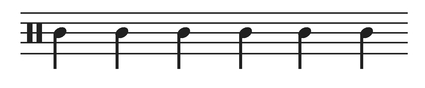
Figure 10.1 Repeating quarter notes.
Time and Rhythm
Peter Martens and Fernando Benadon
Structure is more familiar to us in things we see than in things we hear. We build structures to inhabit; we observe structures in the natural world such as trees or coral reefs. Musical structure is often visible, too; we can see it in the physical movements that produce musical sounds, in the dance moves drawn from musical rhythms, and in the notation used to represent musical ideas. While any of these visible manifestations of musical structure could serve as a useful place to start our treatment of structured musical time, it is perhaps easiest to begin with the visible traces that are captured in standard music notation.
Consider the snippet of music below, a simple string of quarter notes, continuing infinitely (Figure 10.1). No pitch, timbral, or tempo information is given, simply unspecified events occurring in a particular sequential relationship.
Though they may look identical on the page, our understanding of these quarter notes morphs as they proceed in time. Our minds are built to predict the future, to extrapolate probabilities for possible future events based on past experience, and we do this unconsciously with all manner of stimuli (Huron, 2006, p. 3). If we’ve seen three ants emerge from a hole in the ground, we expect more to follow; this is a “what” expectation, and so we would be surprised if an earwig emerged next. Likewise, if we’ve heard five evenly-spaced drips from a leaky faucet hit the sink bottom, we expect more drips to occur with the same time interval between them. This is both a “what” and “when” expectation; we would be surprised by a large delay before drip number six, but we would also be surprised by a finger snap at the exact time that that sixth drip should occur.
These basic habits have a biological foundation (see Henry & Grahn, this volume). Successfully predicting the timing and type of future events confers significant survival advantage to an organism, and the auditory system—operating as it does in full 360° surround—is one of (if not the) most important sensory inputs in terms of this advantage. We bring these habits and reflexive skills to music listening. Returning to Figure 10.1, after we hear only the first two quarter notes we expect a third event to follow the second at the same time interval that separated the second from the first (Longuet-Higgins & Lee, 1982). More precisely, we expect the beginning, or onset, of the third note to correspond to the time span established by the onsets of notes one and two. This span of time from onset to onset, or attack point to attack point, is often referred to as an interonset interval, or IOI. A single IOI is bounded by two events, and thus while two events make us expect a third event, just one IOI makes us expect future similar IOIs. In either way of referring to events in our environment, our minds grab hold of a periodicity: a sequence of temporally equidistant onsets.
Figure 10.1 Repeating quarter notes.
Continuing our thought experiment with Figure 10.1 a step further, if the expectation of a third in-time note (or second equivalent IOI) is met, we have an even stronger expectation of yet another note/IOI with the same spacing in time as the previous, and so on. As the periodic sequence unfolds and our expectations are further validated, our ability to predict the timing of upcoming events is reinforced. This basic ability allows us to synchronize physical movements with other humans (as when playing in a band) or with the sound waves emanating from speakers or headphones (as when moving to a beat). The terms beat induction and entrainment are commonly used for this phenomenon, which may occur at a cognitive or neural level without physical manifestation (Honing, 2013).
Our minds are not content to grasp this single periodicity, however. Once we hear events 1–3, a longer time interval becomes established between events 1 and 3 that leads us to expect event 5 further into the future, while at the same time expecting event 4 immediately next. Event 5 is now expected as a part of two hierarchically organized, or stacked periodicities: the original event string 1,2,3,4,5 and the slower moving event string 1,3,5. Being inextricably linked, these two simultaneous layers of events complement each other’s temporal expectations and increase our anticipation of event 5, as shown by the arrows in Figure 10.2.
It is important to note that we form these expectations unconsciously, and that by default we tend to nest layers by aligning each event in the faster layer with every other event in the slower layer, as in Figure 10.2 (Brochard, et al., 2003). Listening to a dripping faucet or undifferentiated metronome clicks, we naturally impose a grouping, often duple, on the acoustically identical events, even from infancy (Bergeson & Trehub, 2005).1 Any grouping of multiple events into larger time spans is a way to sharpen and heighten our precision as we predict when future events will occur, and these groupings also function to lower the cognitive load by “chunking” a larger number of events in the incoming information stream into fewer discrete units (cf. Zatorre, Chen, & Penhune, 2007).
This nesting of shorter time spans within larger time spans, as conveyed by the brackets and arrows in Figure 10.2, can be applied recursively to include more than just two layers, as long as each event in a slower periodicity is simultaneously a part of all faster periodicities. Thus, our expectations develop over longer time spans in an orderly fashion, for instance, expecting a future 9th quarter note as part of three layers: 1,2,3,4,5,6,7,8,9 (original), 1,3,5,7,9 (half as fast), and 1,5,9 (four times slower than the original). As we will see below, this nesting process will not accrue indefinitely, but in this way we invest some moments in the future with greater “expectational weight” than others. We expect the 9th quarter note more strongly than the 8th, for example, because that 9th quarter note would fulfill the expectations of all three levels of periodicity. The 8th quarter note—at least in this musically impoverished abstraction—only serves to continue the original note-to-note periodicity.
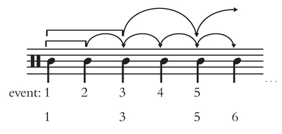
Figure 10.2 Projection and accrual of temporal expectations.
The emergent pattern of expectational peaks, foothills, and valleys brought about by layers of nested expectations gives rise to what we experience as meter in music (Jones, 1992), and is encoded in music notation via a number of symbolic systems such as time signatures and note durations. When we speak of stronger or weaker beats in music, then, we are projecting the products of our own psychological processing onto a musical sound-scape. It is often fairly easy to recognize these patterns when analyzing music, whether notated or not, and so we can speak of a piece’s metric hierarchy when referring to the typical strong-weak patterns of common meters. In 4/4 time, for example, we generally experience beat 1 as the “strongest” in each measure, followed by beat 3, and then beats 2 and 4 about equally.
There are few musical terms used more commonly, yet less precisely, than beat and tempo. We have just used “beat” in the discussion above to refer to each of the four beats in a measure of 4/4 time. This usage implies that the beat in a measure of 4/4 corresponds to the notated quarter note, which is generally true. In terms of cognition, however, we define a beat without recourse to a notated meter, as a periodicity in music onto which we latch perceptually. But already we have two uses of the same term; a beat can refer to a single layer of motion in music (e.g. “this piece has a strong quarter-note beat”), while at the same time we use beat to label each occurrence within that string of events (e.g. “the trumpet enters on beat 4”). To use the term in either sense presupposes a process called beat-finding, whereby the listener infers a consistently articulated periodicity from the music, even if not all beats correspond to sounded events. Evidence for beat-finding can be seen in physical movements such as foot tapping or head nodding in synchrony with the music, and appears to be an almost exclusively human trait (cf. Patel et al., 2009).
Tempo is another term ubiquitous in music that is used in inconsistent and poorly defined ways. Let’s return to Figure 10.1 for a moment. If that rhythm’s speed is not too fast or too slow, each quarter note will be perceived as a beat, and that beat will establish the tempo of the music. We often think of tempo as corresponding to a single periodicity, typically expressed by musicians as beats per minute (BPM). However, as we saw earlier, the basic periodicity of our example gives rise to other nested (slower) periodicities. Further, real music is rarely as simple as a bare string of quarter notes. These two points lead to a key question. Of the several periodicities we can perceive as a beat even in a simple string of identical events, which of them would we define as determining a piece’s tempo? The simplest notion of beat and tempo revolves around the idea of an optimal range for tempo, centered on 100 BPM (Parncutt, 1994) or 120 BPM (Van Noorden & Moelants, 1999). While this turns out to be a complicated issue in fully musical contexts, we can make some general observations about the main beat in the well-known melody shown in Figure 10.3. If we were to hear that melody performed at = 120 BPM, most listeners would latch onto the quarter note as their beat, and would likely describe their experience of tempo in the piece as moderate. If the same melody were performed at = 200 BPM, however, many listeners would instead latch onto the half note at 100 BPM as their beat rate. This brings us to a curious paradox: While our perceived beat would be objectively slower in the second hearing, our judgment of tempo would likely be faster—bouncy or lively (or maybe even too fast!) instead of moderate.
Most commonly, tempo is used by composers, performers, DJs, etc. to refer to the BPM rate of the beat level, often designated as a metronome marking (e.g. mm = 120). Such markings are one way to convey compositional intent in a score or piece of sheet music, or to compare one piece to another as in a BPM table when constructing a set of electronic dance music. Yet BPM rates do not necessarily correspond to a sensation of faster or slower, and this mismatch is the subject of several in-progress research projects. Judgments of tempo are often based on a more general sense of event density (e.g. Bisesi & Vicario, 2015)—how “busy” the musical texture is—and are often encoded by subjective verbal descriptors such as “lively” or “moderate,” or by traditional Italian terms such as “largo” or “allegro con brio.” But even the composer Beethoven found the imprecision of these terms problematic, leading him to champion the objectivity of BPM rates and the newly invented metronome in the early nineteenth century (Grant, 2014, pp. 254ff.).

Figure 10.3 F. J. Haydn, “Austrian Hymn.”
Our minds and bodies are constantly searching our environments for periodic information, and when it exists we attempt to synchronize with these periodicities neurally and physiologically (Merchant et al., 2015). Our initial phase of synchronization with complex periodic stimuli such as music begins at an initial beat or tactus. London (2012, pp. 30–33) cites several hundred years of historical acknowledgement of the concept of tactus, and Honing (2012) argues that at least beat-finding (if not meter-finding) is innate, a basic and constant cognitive operation when listening to music.
While we might assume that the tactus in Figure 10.1 is obvious—it’s a string of quarter notes, after all—beat-finding is constrained and directed by several salience criteria that serve to mark some musical attacks for attention over others. All such criteria lend accentual weight to these moments, and these accents can come from harmony (the tonic triad feels more stable than other chords), melody (a particularly high or long note stands out), instrumentation (a snare drum attack is prominent in many textures), articulation (a violinist’s martelé bow stroke marks notes for attention), and the list could go on. Both Lerdahl and Jackendoff (1983) and Temperley (2001) construct theoretical models for meter perception that attempt to account for these various factors, albeit in more general ways, in the form of metrical preference rules (MPRs). For instance, Temperley’s MPR 6 states that we “prefer to align strong beats with changes in harmony” (p. 51), while Lerdahl and Jackendoff’s MPR 7 states that we “Strongly prefer a metrical structure in which cadences are metrically stable” (p. 88). In addition to the perceptual cues that accentual markers provide, the particular distribution of accented onsets affects how a listener assigns a specific “internal clock” that most efficiently matches the pattern of the heard rhythm (Povel & Essens, 1985).
Despite the above models’ recognition of the importance of a tactus level, what is perhaps the most basic cognitive factor in beat-finding is left under-theorized: tempo. London (2012) summarizes relevant research and creates “Tempo-Metrical Types” that map out the ramifications of tempo for not just tactus but for entire metric structures. Imagine “Flight of the Bumblebee”; now imagine tapping your foot along to each note—impossible! Even though we perceive each note as part of the melody, that periodicity is simply too fast to suggest a beat (defined as beat perception ) and too fast to match physically (defined as beat production ). When periodic events are faster than roughly 250 ms (240 BPM), we tend to hear them not as a beat (main or otherwise), but as divisions and subdivisions (i.e., divisions of divisions) of a slower moving periodicity. If our “Flight of the Bumblebee” melody notes are speeding along at 120 ms (500 BPM), as is typical, we will likely group four attacks per beat and synchronize with the music at the more comfortable rate of 480 ms (125 BPM). On the other end of the tempo spectrum, at rates slower than about two seconds (30 BPM) our production accuracy plummets, and perception suffers as well. Lacking intervening events, we increasingly perceive very slow events as disconnected—still sequential in time, but not periodic.
There is a large and fairly well-defined range of beat interonset values—250 to 2,000 ms, or 30 to 240 BPM—within which beats can emerge. As noted above, some research has pointed to a tempo “sweet spot” in the middle of this tempo window, anywhere from 100 to 140 BPM. These findings, however, were largely extrapolated from empirical studies that elicited physical responses to metronome clicks or other musically impoverished stimuli, an issue of ecology when the behavior under investigation is music listening. In empirical studies using excerpts of real music, beat-finding is often assessed using a similar procedure, asking subjects to tap along with the stimuli; verbal directions in these studies often steer subjects toward the most salient or most comfortable pulse rate in the music. These studies present a more complex picture of meter perception: in addition to the multivalent salience factors present in the music itself, the unique habits and experiences of individual listeners have also been found to be a factor (see Repp & Su, 2013). For example, McKinney and Moelants (2006) found that accent patterns in music from a variety of styles could cause listeners to choose a tapped tactus as slow as 50 BPM and as fast as 220 BPM, and found considerable differences between individual subjects. Martens (2011) theorized a tripartite characterization of individual subjects’ beat-finding behaviors based on their preferred beat’s degree of nesting within a metric hierarchy, and suggested that the specifics of subjects’ musical experience and training (e.g., type of instrument played, years of formal training) might play a role in an individual’s beat-finding strategy.
While it is difficult to predict a specific preferred beat percept across individuals and musical situations, there are musical styles in which there may be broad, even uniform agreement about which of the nested periodicities carries the beat. One such musical genre is dance-oriented pop/rock music from about 1950 onward, music that typically contains an alternation of bass drum and snare drum at a moderate tempo of 90–130 BPM. Inherently attractive due to tempo alone, this 4/4 “backbeat” pattern, with bass drum attacks on beats 1 & 3 and snare attacks on beats 2 & 4, clearly defines the tactus in much Western popular music. If the purpose of the music is coordinated group movement like dancing, it only makes sense that the tactus of such music will be strongly felt. 2 Regardless of musical style, once we synchronize to an initial beat can we begin to explore a multi-layered meter by moving to faster or slower beats due to continued metric foraging. Jones and Boltz (1989) propose a model of “dynamic attending” whereby listeners shift their attention and/or movements from a tactus to faster or slower beats, whether in response to subtle changes in the music or the physical, mental, or emotional needs of the moment.
If we explore a piece’s metric hierarchy from the anchoring periodicity of our initial beat, the most obvious choices from a perceptual perspective are the periodicities immediately faster and slower than that beat rate—divisions and groupings, respectively. This basic multilayered conception of meter cognition is built into Western notation. See Table 10.1. In this outlay of typical meter or time signatures, the existence of a main beat or tactus is assumed. The three columns reflect possible groupings of that beat in twos, threes, and fours, while the two rows reflect divisions of that beat into two (simple) or three (compound). 3 Different meters of the same general type (i.e., having the same division and grouping) have been used historically for different stylistic or genre-based reasons, but they share basic perceptual characteristics.
A central assumption of the metric framework explored above is that it conforms to an isochronous grid. This assumption stipulates that all note values bearing the same name also have the same duration: for example, all sixteenth notes are equal. Despite its explanatory power, the metric model appears to be at odds with the fact that music is often played with little regard to
Table 10.1 Common meter signatures arranged by type.
| duple beat grouping | triple beat grouping | quadruple beat grouping | |
| simple beat division | 2 2 | 3 3 3 | 4 4 4 |
| 4 2 | 8 4 2 | 8 4 2 | |
| compound beat division | 6 6 | 9 | 12 |
| 8 4 | 8 | 8 |
strict isochrony (Seashore, 1938). In contrast to the rigid evenness of the metric grid, analysis of performance timing—also known as microtiming, expressive timing, or rubato—reveals widespread non-isochrony in a wide range of repertoires, including Western classical music (Povel, 1977), Mozambiquean xylophone duos (Kubik, 1965), Cuban drumming (Alén, 1995), Swedish folk music (Bengtsson & Gabrielsson, 1983), and American jazz (Ashley, 2002).
Timing inflections are often a function of a performer’s individual preferences (Repp, 1992a). Figure 10.4 shows timing information for two different recordings of the same excerpt; interonset intervals for each violinist are plotted on the y-axis. Whereas the graph of an isochronous performance would look like a flat horizontal line, these renditions contain some temporal variance, each outlining a distinct contour. In contour A, there is a durational peak occurring on the fifth note, highlighting the perceptual importance of the measure downbeat (and its associated V7 -I harmonic resolution). Timing can therefore interact with meter irrespective of isochrony. A different kind of timing-meter interaction can be seen in contour B, where the start of each four-note group is emphasized with a mild elongation. Both cases underscore the notion that timing is often closely linked to grouping structure, as exemplified by the characteristic deceleration known as phrase-final lengthening (Todd, 1985).
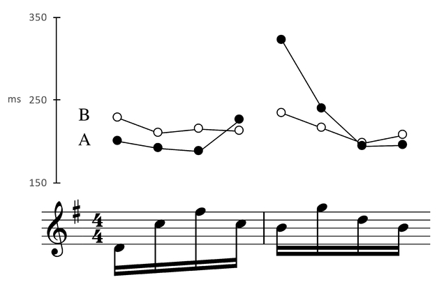
Figure 10.4 Timing contours for two different violinists, from Haydn Op. 76/3, Mvt. 2. A = Erich Höbarth (Quatuor Mosaï ques), B = Norbert Brainin (Amadeus Quartet).
The link between timing and grouping structure is not confined to production, but involves perception as well. Repp (1992b) presented listeners with classical piano excerpts that had been altered to lengthen certain notes within an otherwise isochronous texture. Participants had more difficulty detecting the note elongations when they occurred at structurally salient moments. Since the expectation was that a performer would normally apply some degree of local deceleration at precisely those moments, the magnitude of the artificial alteration in the stimuli’s corresponding notes had to be particularly prominent in order for participants to detect it. Structure “warped” the listener’s mental timekeeper. Interestingly, detection accuracy scores were not strongly correlated with musical training or familiarity with the repertoire. In a later replication, Repp (1999) suggested that the ability of musically untrained participants to perform the detection task comparably to trained musicians could be attributed to innate perceptual skills. What is certain is that the cognitive implications of performance timing depend in large part on the magnitude of the effect. While most listeners can likely detect the spike in Figure 10.4’s contour A, the fluctuations in B are more understated—perhaps more felt than heard, such that their absence would rob the performance of some of its underlying expressivity. Honing (2006) has shown that experienced listeners are sensitive to the subtle expressive timing changes that result from altering a recording’s tempo. Presented with pairs of recordings of the same composition (one of which had been digitally transformed to match the tempo of the other rendition), participants correctly identified the recording that had been left intact. This ability to pick up on relative and presumably subliminal timing cues was later shown by Honing and Ladinig (2009) to be enhanced by prior exposure to the genre of the presented recordings. Timing perception is shaped by both biology and enculturation.
To understand why metric structure does not break down in the face of non-isochrony, it helps to think of note durations as determined categorically rather than by fixed absolute values. In a study by Desain & Honing (2003), expert musicians used music notation to transcribe a variety of aurally presented three-note rhythms. Even though most of the rhythms featured complex interonset ratios, these tended to be consistently “clumped” by transcribers into a small number of simpler rhythmic categories. For instance, almost all participants notated the rhythm 1.8:1:1 as a quarter-note followed by two eighth-notes, the equivalent of 2:1:1. The study’s second experiment repeated the same procedure, but now the rhythms were immediately preceded by two measures divided into either two or three isochronous notes, thus suggesting either duple or triple meter. The metric priming affected the category boundaries, leading participants to use duple-meter transcriptions 99% of the time when the prime was duple but only rarely when the prime was triple.
Context is therefore a key factor in how timing patterns are processed. In Figure 10.4, violinist A’s notes are heard as categorically equivalent—as sixteenth notes—even though the fifth note is drastically longer than the rest. By this point in the passage, the listener has inferred a metric scaffold whereby four sixteenth notes group into beats, which in turn group into 4/4 measures. It would be unwise in terms of cognitive efficiency to topple this perceptual tower by interpreting the lengthened note as anything but a sixteenth note.
While categorical perception helps us reconcile the abstract isochrony of meter with the realized non-isochrony of performance, in some instances this reconciliation is more elusive. In an isochronous setting, the second of a beat’s two eighth notes lies halfway along the beat – both eighths have the same duration, represented as a binary 1:1 ratio. If the same beat is instead subdivided so that the first note is twice as long as the first, the result is a ternary 2:1 ratio (a triplet quarter note followed by a triplet eighth note). These ratios need not be exact in order for either category—binary or ternary—to emerge, so that, for example, 1.9:1 still sounds ternary (Clarke, 1987). However, the category boundary is fuzzy enough that a slightly longer first eighth note (roughly between 1.2:1 and 1.5:1) creates a particular rhythmic “feel” that is neither clearly binary or clearly ternary. This kind of categorical ambiguity is prevalent across multiple musical traditions and has been extensively documented in jazz (Benadon, 2006) and African drumming (Polak & London, 2014).
If rhythms are patterns of events in sounded music that can be imprecise, expressive, and messy, while meter is a quantized mental construct of regular nested periodicities, how do the two interact during a music listening experience? As we listen over longer spans of time, Lerdahl and Jackendoff (1983, p. 36) point out that we automatically segment or chunk music into informal structural units of varying sizes (e.g. phrases, themes, or motives) in the same way that we group events or items of any kind (e.g. the things in my pocket, or people I’ve seen today) (cf. Temperley, 2001, p. 55ff. for a more thorough discussion). These segments, or rhythmic groups, are independent of metric groups (e.g. measures), although the two are frequently coterminous.
Both types of groups are grasped in time, as they develop. The steady quarter notes of Figure 10.1 represent a rhythmic group, albeit a rather boring one, that causes us to perceive an analogous steady beat that accrues into metric groups. The rhythms in the Haydn and Beethoven melodies shown in Figures 10.3 and 10.5, respectively, give rise to metrical percepts very similar to those formed by Figure 10.1, even though the rhythms of both melodies are less regular and more complex. What accounts for the different rhythmic feel of musical melodies versus repeated quarter notes? Lacking any additional information, the first event of a rhythmic group will be invested with the weight of a strong metrical beat (cf. Temperley, 2001, MPR 4, p. 32; Lerdahl & Jackendoff, 1983, MPR 2, p. 76). In the quarter notes of Figure 10.1 and the Haydn melody, the rhythmic group begins with the first quarter note, as does our perceived meter. In Beethoven’s melody, by contrast, the bracketed rhythmic groups are offset from groups of metrical events (i.e., measures), as indicated by brackets in Figure 10.5. Our judgments about that melody’s pitch relationships, melodic contour, and relative note durations combine to suggest that the beginning of this rhythmic group does not initiate a metrical group, and instead forms a series of pickup notes. When listening to the Beethoven melody, then, our basic procedure of grouping produces segments that are offset from the segments of meter.
In both simple and complex musical contexts, sounding rhythms give rise to a perception of meter. Even though meter is in this way dependent upon rhythm, the periodic expectations of meter can and will persist for a while if rhythmic support disappears, or in the face of rhythmic input that conflicts with an established meter. This relationship accounts for the phenomenon of “loud rests” (London, 2012, p. 107) and other silent moments in music at time points when we were expecting something to occur. Snyder and Large (2005) collected electroencephalography (EEG) data that showed undiminished neural activity in response to repeated loud-soft tone sequences when either a single loud or soft tone was occasionally omitted; in this way metrical patterns are literally mimicked by the brain, which will continue them (if only briefly) on its own. The interplay between events in the sounding music (i.e., rhythms) and an established set of metric expectations provides one basis for the basic psychological effects of music, first theorized by Meyer (1956) and notably refined and expanded by Huron (2006). Yet in terms of musical time, there is a paradox; as described above, sounding rhythms created those metric expectations in the first place.
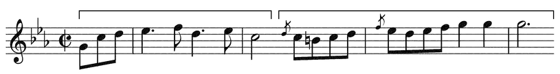
Figure 10.5 L. van Beethoven, theme from Piano Sonata Op. 13, Mvt. 3 with brackets showing rhythmic groups offset from metrical units (barlines).
The perceptual balance between rhythm and meter is a delicate one. Two possible rhythm-meter cycles are shown in Figure 10.6. Figure 10.6A depicts the perceptual loop experienced in music that is consistently metric: there are few or no cross-accents, and thus our metric expectations are not only explicitly confirmed but also renewed. Now imagine that the music begins to bombard us with rhythms that emphasize weak time points in the established meter (such as offbeats or syncopations), or even rhythms that simply emphasize a different beat rate in the existing meter. Figure 10.6B conveys how a metric percept might change during a piece of music in response to conflicting rhythmic information. In these situations, the acoustic stimulus of rhythm reshapes the mental percept of meter (cf. London, 2012, p. 100ff. for an analytical example of this process occurring during music listening).
In highly complex rhythmic contexts, it is not uncommon for listeners—sometimes even the players themselves—to “lose their place” by mistaking beats for upbeats (and vice-versa) or by assigning the measure’s downbeat to the wrong beat.
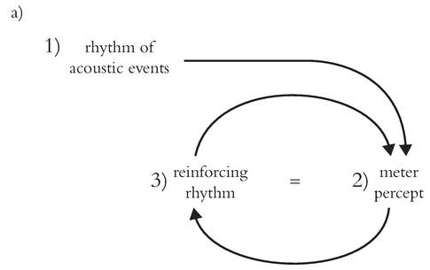
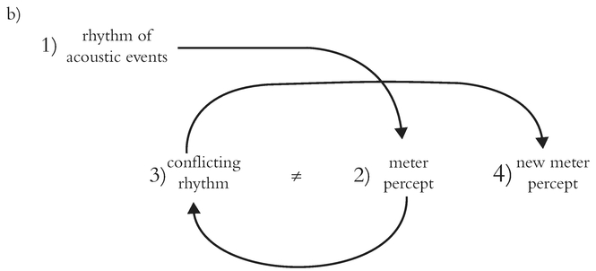
Figure 10.6 Rhythm/Meter cycles: (A) Rhythm establishing meter, meter reinforced by subsequent rhythm. (B) Rhythm establishing meter, meter contradicted by subsequent rhythm, new meter established.
In much of the music performed around the world, we would expect to experience a continuum of relationships between rhythm and meter, with the perceptual options captured in Figure 10.6 functioning as endpoints. We often hear rhythms that briefly suggest or point to a meter other than the one we are currently experiencing, but these rhythms are not sufficiently strong or long-lasting to induce a new metric percept. Indeed, the interplay between rhythm and meter, the gray perceptual area between Figure 10.6A and B, is an essential spice of musical time. If our expectations are consistently met by highly predictable rhythms, we can lose interest and push the music to the background of our attention—this can actually be an intentional compositional strategy in music intended as “acoustic wallpaper.” Conversely, if a string of musical rhythms gives us no periodic information from which to predict future events, we may also lose interest, unconsciously deeming the music biologically unhelpful, and turn our attention elsewhere. These aesthetic responses are a musical manifestation of “subjective complexity,” one dimension of an individual’s musical taste (cf. Lamont & Greasley, 2009).
The boundary between these processes, and indeed the process itself shown in Figure 10.6B, has received little empirical attention. While the amount of literature on the perception and cognition of rhythm and meter has exploded during the past 40 years, it should perhaps not be surprising that, given such a complex set of relevant physiological and psychological processes, matched by an equally complex set of musical possibilities, this area of study is only approaching adolescence. Further, identifying and describing the procedures by which we apprehend time in music is only a first step in coming to understand what, and how, music means to us—the reason so many of us are drawn to music in the first place. As our cognitive faculties continually assess incoming temporal information for regularities, the manipulation of time in the structure or performance of musical rhythms is a potent means to musical meaning, a significant tool in the kit of composers and performers across musical styles, cultures, and epochs.
1. Of course, our preference for duple grouping does not preclude other groupings, with triple groupings certainly being common in some musical contexts. The propensity for one or another grouping is possibly affected by enculturation (cf. Hannon & Trehub, 2005).
2. This is not the same, however, as saying that the tactus must be strongly articulated; cf. Butler (2006) for the idea that omitting attacks from the tactus level actually invites dancers to supply the “missing” tactus level with their physical movements.
3. Diverse musical traditions may have less regular patterns of beat grouping or division, and these also exist in the Western tradition as “mixed” or “asymmetrical” meters.
Desain, P., & Honing, H. (2003). The formation of rhythmic categories and metric priming. Perception, 32, 341–365.
Honing, H. (2013). Structure and interpretation of rhythm in music. In D. Deutsch. (Ed.) The psychology of music (3rd ed.) (pp. 369–404). London: Academic Press.
Jones, M. R. (2009). Musical time. In S. Hallam, I. Cross, & M. Thaut (Eds.) The Oxford handbook of music psychology (pp. 81–92). Oxford: Oxford University Press.
Lerdahl, F., & Jackendoff, R. (1983). A generative theory of tonal music. Cambridge, MA: MIT Press.
London, J. (2012). Hearing in time. Oxford and New York, NY: Oxford University Press.
Repp, B., & Su, Y. (2013). Sensorimotor synchronization: a review of recent research (2006–2012). Psychonomic Bulletin Review, 20(3), 403–452.
Temperley, D. (2001). The cognition of basic musical structures. Cambridge, MA: MIT Press.
Alén, O. (1995). Rhythm as duration of sounds in Tumba Francesa. Ethnomusicology, 39(1), 55–71.
Ashley, R. (2002). Do[n’t] change a hair for me: The art of jazz rubato. Music Perception, 19(3), 311–332.
Benadon, F. (2006). Slicing the beat: Jazz eighth-notes as expressive microrhythm. Ethnomusicology, 50(1), 73–98.
Bengtsson, I., & Gabrielsson, A. (1983). Analysis and synthesis of musical rhythm. In J. Sundberg (Ed.), Studies of Music Performance. (No. 39) (pp. 27–60). Stockholm: Royal Swedish Academy of Music.
Bergeson, T., & Trehub, S. (2005). Infants’ perception of rhythmic patterns. Music Perception, 23(4), 345–360.
Bisesi, E., & Vicario, G. B. (2015). The perception of an optimal tempo: The role of melodic event density, in A. Galmonte & R. Actis-Grosso. (Eds.), Different psychological perspectives on cognitive processes: Current research trends in Alps-Adria region, (pp. 25–43). Cambridge: Cambridge Scholars Publishing.
Brochard, R., Abecasis, D., Potter, D., Ragot, R., & Drake, C. (2003). The “ticktock” of our internal clock direct brain evidence of subjective accents in isochronous sequences. Psychological Science, 14(4), 362–366.
Butler, M. (2006). Unlocking the groove: Rhythm, meter, and musical design in electronic dance music. Bloomington, IN: Indiana University Press.
Clarke, E. (1987). Categorical rhythm perception: An ecological perspective. In A. Gabrielsson (Ed.), Action and Perception in Rhythm and Music (No. 55) (pp. 19–33). Stockholm: Royal Swedish Academy of Music.
Grant, R. M. (2014). Beating time and measuring music in the early modern era. Oxford: Oxford University Press.
Hannon, E., & Trehub, S. (2005). Tuning in to musical rhythms: Infants learn more readily than adults. Proceedings of the National Academy of Sciences, 102(35), 12639–12643.
Honing, H. (2006). Evidence of tempo-specific timing in music using a web-based experimental setup. Journal of Experimental Psychology: Human Perception and Performance, 32(3), 780–786.
Honing, H. (2012). Without it no music: Beat induction as a fundamental musical trait. Annals of the New York Academy of Sciences, 1252, The Neurosciences and Music IV – Learning and Memory, 85–91.
Honing, H., & Ladinig, O. (2009). Exposure influences expressive timing judgments in music. Journal of Experimental Psychology: Human Perception and Performance, 35(1), 281–288.
Huron, D. (2006). Sweet anticipation: Music and the psychology of anticipation. Cambridge, MA: MIT Press.
Jones, M. R. (1992). Attending to musical events. In M. R. Jones and S. Holleran (Eds.), Cognitive bases of musical communication (pp. 91–110). Washington, DC: American Psychological Association.
Jones, M. R., & Boltz, M. (1989). Dynamic attending and responses to time. Psychological Review, 96(3), 459–491.
Kraemer, D. J. M., Macrae, C. N., Green, A. E., & Kelley, W. M. (2005). Musical imagery: Sound of silence activates auditory cortex. Nature, 434 (7030), 158.
Kubik, G. (1965). Transcription of Mangwilo xylophone music from film strips. African Music, 3(4), 35–51.
Lamont A., & Greasley, A. E. (2009). Musical preferences. In Hallam, S., Cross, I., Thaut, M. (Eds.) Oxford handbook of music psychology. (pp. 160–168). Ne w York, NY: Oxford University Press.
Longuet-Higgins, H. C., & Lee, C. S. (1982). The perception of musical rhythm. Perception, 11, 115–128.
Martens, P. (2011). The ambiguous tactus: Tempo, subdivision benefit, and three listener strategies. Music Perception, 28, 433–448.
McKinney, M. F., & Moelants, D. (2006) Ambiguity in tempo perception: What draws listeners to different metrical levels? Music Perception, 24, 155–166.
Merchant, H., Grahn, J., Trainor, L., Rohrmeier, M., & Fitch, W.T. (2015). Finding the beat: A neural perspective across humans and non-human primates . Philosophical Transactions of the Royal Society B, 370, 20140093.
Meyer, L. (1956). Emotion and meaning in music. Chicago, IL: University of Chicago Press.
Parncutt, R. (1994). A perceptual model of pulse salience and metrical accent in musical rhythms. Music Perception, 11(4), 409–464.
Patel, A., Iversen, R., Bregman, M., & Schulz, I. (2009). Experimental evidence for aynchronization to a musical beat in a nonhuman animal. Current Biology, 19, 827–830.
Polak, R., & London, J. (2014). Timing and meter in Mande drumming from Mali. Music Theory Online 20(1). http://mtosmt.org/issues/mto.14.20.1/mto.14.20.1.polak-london.html
Povel, D. J. (1977). Temporal structure of performed music: Some preliminary observations. Acta Psychologica, 41, 309–320.
Povel, D. J., & Essens, P. (1985). Perception of temporal patterns. Music Perception, 2(4), 411–440.
Repp, B. (1992a). Diversity and commonality in music performance: An analysis of timing microstructure in Schumann’s “Träumerei.” Journal of the Acoustical Society of America, 92(5), 2546–2568.
Repp, B. (1992b). Probing the cognitive representation of musical time: Structural constraints on the perception of timing perturbations. Cognition, 44, 241–281.
Repp, B. (1999). Detecting deviations from metronomic timing in music: Effects of perceptual structure on the mental timekeeper. Perception and Psychophysics, 61(3), 529–548.
Seashore, C. (1938). Psychology of music. New York, NY: McGraw Hill.
Snyder, J. S., & Large, E. W. (2005). Gamma-band activity reflects the metric structure of rhythmic tone sequences. Cognitive Brain Research, 24(1), 117–126.
Todd, N. (1985). A model of expressive timing in tonal music. Music Perception, 3, 33–58.
Van Noorden, L., and Moelants, D. (1999). Resonance in the perception of musical pulse. Journal of New Music Research, 28(1), 43–66.
Zatorre, R., Chen, J., & Penhune, V. (2007). When the brain plays music: Auditory-motor interactions in music perception and production. Nature Reviews Neuroscience, 8, 547–558.