Assembling a Neural Network from Perceptrons

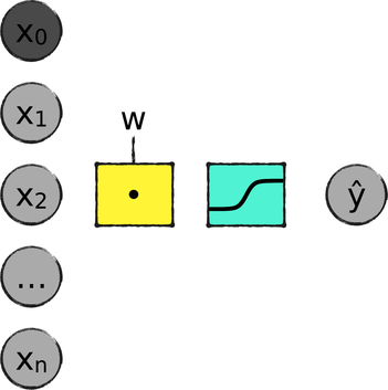
Let’s see how to build a neural network, starting with the perceptron that we already have. As a reminder, here is that perceptron again—a weighted sum of the inputs, followed by a sigmoid:

In Part I of this book, we didn’t just use the perceptron as is—we also combined perceptrons in two different ways. First, we trained the perceptron with many MNIST images at once; and second, we used ten perceptrons to classify the ten possible digits. In ​Assembling Perceptrons​, we compared those two operations to “stacking” and “parallelizing” perceptrons, respectively, as shown in the picture.

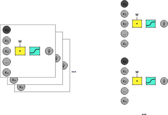
To be clear, we didn’t literally stack and parallelize perceptrons. Instead, we used matrices to get a similar result. Our perceptron’s input was a matrix with one row per image; and our perceptron’s output was a matrix with ten columns, one per class. The “stacking” and “parallelizing” metaphors are just convenient shortcuts to describe those matrix-based calculations.

Now we’re about to take these extended (stacked and parallelized) perceptrons, and use them as building blocks for a neural network.

Chaining Perceptrons

We can build a neural network by serializing two perceptrons like this:

See? Each perceptron has its own weights and its own sigmoid operation, but the outputs of the first perceptron are also the inputs of the second. To avoid confusion, I renamed those values with the letter h, and I used d to indicate their number. h stands for “hidden,” because these values are neither part of the network’s input, nor the output. (And since I know that you’re going to ask: the d stands for nothing in particular. I just took a cue from mathematicians and came up with a random letter.)

Back in the day, a structure like this one was called a multilayer perceptron, or an artificial neural network. These days, most people simply call it a neural network. The round gray bubbles in the network are called nodes, and they’re arranged in layers, as shown in the picture.

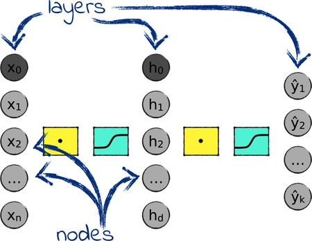
This network has three layers: an input layer, a hidden layer, and an output layer. You can also concatenate more than two perceptron and end up with more than three layers—but we can save that topic for the next part of this book. For now, we’ll focus on three-layered neural networks.

The nodes in the hidden layer are calculated from the nodes in the input layer, except for one node: the bias. When we joined two perceptrons together to create the network, both perceptrons kept their bias node. So now we have a bias node in the input layer, and another in the hidden layer. The values of those nodes are fixed at 1. (If you don’t remember why 1, then review ​Bye Bye, Bias​.)

Let me be clear on what we mean when we say, for example, “this layer has 10 nodes.” That doesn’t mean that the neural network represents that layer as an array of 10 elements—it means that the neural network represents that layer as a matrix of 10 columns, and as many rows as it needs. For example, if we’re training a network on a dataset of 5,000 examples, then the layer will be represented by a (5000, 10) matrix. Just like the diagram of a perceptron, the diagram of a neural network pretends that the network is always processing one example at the time, for the sake of readability. Remember our “stacking” metaphor: when you look at these diagrams, imagine that there are as many networks as we have training examples, stacked upon each other.

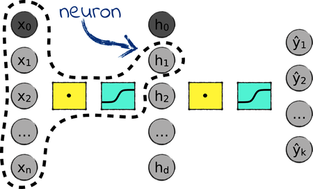
Sometimes, people refer to the nodes in a neural network as neurons. To be precise, a neuron isn’t just a node. It also includes the components that directly impact its value—the nodes in the previous layer, and the operation in between, as illustrated by the picture.

Finally, as I mentioned earlier, the functions in between layers are called the activation functions of the network. In the network that we’re looking at, both activation functions are sigmoids—but that isn’t necessarily the case, as we’ll find out soon.

With that, we know what a three-layered neural network looks like in general. However, we didn’t decide the number of nodes in each layer of our network. Let’s do that.

How Many Nodes?

Let’s see how many nodes we need for our network’s input, hidden, and output layers.

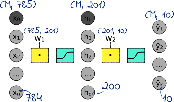
Let’s start with the number of input nodes. Just like a perceptron, our network has an input node for each input variable in the data, plus the bias. We’re looking to classify MNIST’s 784-pixels images, so that makes 785 input nodes. Our input matrix will have one row per image, and 785 columns—the same as the perceptron.

The number of output nodes is also the same as the perceptron’s. There are 10 classes in MNIST, so we need 10 output nodes. The output matrix will have one row per image, and 10 columns.

What about the number of hidden nodes? That one is for us to decide, and in a few chapters we’ll see how to take a smart decision. For now, let’s go with a simple rule of thumb: the number of hidden nodes is usually somewhere between the number of input and output nodes. So let’s set it at 200, that becomes 201 once we add the bias.

You might wonder why I chose an awkward number like 201. After all, the network is likely to perform pretty much the same with one node more or less. So why don’t we start with 199 hidden nodes, and end up with a round 200 after adding the bias? Indeed, we could just as well do that. I opted for 201 as a reminder that one of the hidden nodes is special: it has a fixed value of 1, to take care of the bias.

Finally, let’s talk about the weights. We built our network by chaining two perceptrons, each with its own matrix of weights. As a result, the neural network has two matrices of weights: one between the input and the hidden layer, and one between the hidden and the output layer. We can get their dimensions with a simple general rule: each matrix of weights in a neural network has as many rows as its input elements, and as many columns as its output elements. In other words, w1 is (n, d), and w2 is (d, k). In case you want to check, that rule also applies to the perceptron: the matrix of weights of our perceptron had one row per input variable, and one column per class.

If you find all these matrix dimensions confusing, check them for yourself. Here are the operations in the network:

​	H = sigmoid(X ⋅ W1)
​	Ŷ = sigmoid(H ⋅ W2)

Remember the rules of matrix multiplication from ​Multiplying Matrices​, and also remember that the output of the sigmoid has the same dimensions as its inputs.

Let’s sketch the number of nodes and the matrix dimensions on the network diagram. I will use the letter m to indicate the number of inputs, which can vary. It’s 60,000 in the MNIST training set, but it can be as little as 1 during classification, if we classify a single image:

The plan is looking nice. You’re probably itching to turn it to code—but first, we have one last change to make.