From the Chain Rule to Backpropagation

Backpropagation is an application of the chain rule, one of the fundamental rules of calculus. Let’s see how the chain rule works on a couple of network-like structures: a simpler one, and a more complicated one.

The Chain Rule on a Simple Network

Look at this simple network-like structure:

This one isn’t a neural network, because it doesn’t have weights. Let’s borrow a term from computer science, and call it a computational graph. This graph has an input a, followed by two operations: “multiply by two” and “square.” The output of the multiplication is called b, and the output of the entire graph is called c.

Now let’s say that we want to calculate ∂c/∂a, the gradient of c with respect to a. Intuitively, that gradient represents the impact of a on c: whenever a changes, c also changes, and the gradient measures how much. (If this way of thinking about the gradient sounds perplexing, then maybe review ​Gradient Descent​.)

For such a small graph, we could calculate ∂c/∂a in a single shot, by taking the derivative of c with respect to a. As we mentioned earlier, however, that derivation would become impractical for very large graphs. Instead, let’s calculate the gradient using the chain rule, that works for graphs of any size.

Here is how the chain rule works. To calculate ∂c/∂a:

1. Walk the graph back from c to a.

2. For each operation along the way, calculate its local gradient—the derivative of the operation’s output with respect to its input.

3. Multiply all the local gradients together.

Let’s see how that process works in practice. In our case, the path back from c to a involves two operations: a square and a multiplication by 2. Let’s jot down the local gradients of those two operations:

How do I know that ∂b/∂a is 2, and ∂c/∂b is 4a? Well, even though we’re using the chain rule, we must still compute the local gradients in the old-fashioned way, taking derivatives by hand. However, don’t fret if you don’t know how to take derivatives—there are libraries that do that. Just understand how the process works, and you’re golden.

Now that we have the local gradients, we can multiply them to get ∂c/∂a:

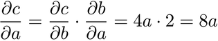
So, there’s our answer, courtesy of the chain rule: the gradient of c with respect to a is 8a. In other words, if a changes a little, then c changes by 8 times the current value of a.

To recap the chain rule: to calculate the gradient of any node y with respect to any other node x, we multiply the local gradient of all the nodes on the way back from y to x. Thanks to the chain rule, we can calculate a complicated gradient as a multiplication of many simple gradients.

Now let’s look at a computational graph that’s a bit more similar to a neural network.

Math Deep Dive: The Chain Rule
	If you watched Khan Academy’s screencasts on calculus, then you might already have seen the videos on the chain rule.[17] As usual, this material goes deeper than you need for the purposes of reading this chapter—but if you like math, it’s definitely worth a watch.

Now For Something More Complicated…

The name “backpropagation” is a shorthand for “calculate the gradients of a neural network’s loss with respect to the weights using the chain rule.” As an example, check out this second computational graph.

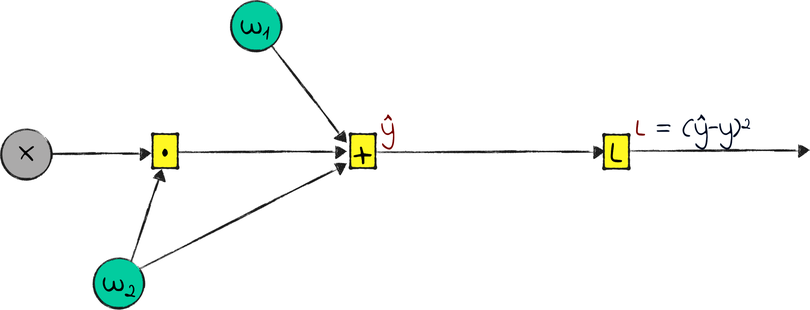
This graph is not going to win any ML competitions. In fact, you might argue that it’s not even a neural network. However, it has what it takes to stand for a neural network in this example: an input x, an output ŷ, and a couple of weights. It also has a loss L, calculated as the squared error of the difference between ŷ and the ground truth y.

Imagine freezing this network mid training, right before the next step of gradient descent. Let’s say that w₁ and w₂ are currently 6 and 2. Also, let’s say that we only have one training example, that has x = 3 and y = 17. From those numbers, we can calculate the other values in the graph:

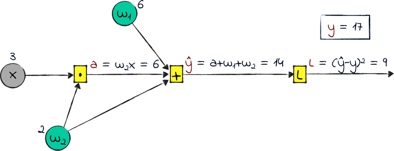
I didn’t have a name for the output of the multiplication, so I called it a.

To take a step of GD, we need the gradients of L with respect to w₁ and w₂. We can compute those gradients with the chain rule. Remember how it works? ∂L/∂w₁ is the product of the local gradients on the way back from L to w₁. The same goes for ∂L/∂w₂. Let’s get down to business and calculate those local gradients.

Note that this graph has an added difficulty compared with the one from the previous section: some operations have multiple inputs. If an operation has multiple inputs or outputs, then we have to calculate its local gradient for each input–output pair. Taking that fact into account, we need five local gradients. Here they are, complete with their numerical values:

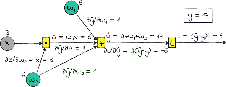
Now we can apply the chain rule. First, let’s calculate ∂L/∂w₁. If you wanted to be precise, you could read that gradient as “the gradient of L with respect to w₁”—but because that’s a mouthful, machine learning practitioners tend to call it “the gradient of w₁” for short.

To get the gradient of w₁, we multiply all the gradients between L and w₁:

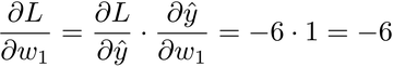
There you have it: with the current weights, the gradient of w₁ is -6. To take the next step of GD, we would multiply this gradient by the learning rate, and subtract the result from w₁.

We can follow a similar process to get ∂L/∂w₂, although in this case we have an additional complication: there are two paths leading from w₂ to L—one that passes by the multiplication, and one that doesn’t. Whenever we have multiple paths, we have to sum their gradients:

∂L/∂w₂ is also negative, but larger than ∂L/∂w₁. Once again, we can multiply this gradient by the learning rate, and subtract the result from w₂.

You can see ∂L/∂w₁ and ∂L/∂w₂ as measures of how much each weight is contributing to the loss. Both weights have a negative contribution, meaning that they must grow so that the loss gets smaller. However, w₂ is contributing more than w₁, because it’s involved twice in the calculation of ŷ—once in the multiplication, and once in the sum.

In general, if a weight has a small gradient, that means that it doesn’t contribute much to the network’s error, so it can change just a little bit. Conversely, a weight with a large gradient is having a big impact on the network’s error, and needs to be changed more decisively. Backprop is a way to calculate how much each weight needs to change.

We just applied backpropagation—an algorithm to calculate the gradients of the weights by multiplying the local gradients of individual operations. It’s called backpropagation because, conceptually, it moves in the opposite direction of forward propagation. Forward propagation moves from the inputs to the outputs, and ultimately calculates the loss; backpropagation moves back from the loss to the weights, accumulating local gradients through the chain rule.

Now that we have a grip on backpropagation, let’s apply it to our network.