Initializing the Weights
Let me wax nostalgic about perceptrons for a moment. Back in Part I of this book, weight initialization was a quick job: we just set all the weights to 0. By contrast, weight initialization in a neural network comes with a hard-to-spot pitfall. Let’s describe that pitfall, and see how to walk around it.
Fearful Symmetry
Here is one rule to keep in mind: never initialize all the weights in a neural network with the same value. The reason for that recommendation is subtle, and comes from the matrix multiplications in the network. For example, look at this matrix multiplication:

You don’t need to remember the details of matrix multiplication, although you can review Multiplying Matrices if you want to. Here is the interesting detail in this example: even though the numbers in the first matrix are all different, the result has two identical columns, because of the uniformity of the second matrix. In general, if the second matrix in the multiplication has the same value in every cell, the result will have the same values in every row.
Now imagine that the first and second matrices are respectively x and w₁—the inputs and the first layer’s weights of a neural network. Once the multiplication is done, the resulting matrix passes through a sigmoid to become the hidden layer h. Now h has the same values in each row, meaning that all the hidden nodes of the network have the same value. By initializing all the weights with the same value, we forced our network to behave as if it had only one hidden node.
If w₂ is also initialized uniformly, this symmetry-preserving effect happens on the second layer as well, and even during backpropagation. In the “Hands On” section at the end of this chapter, we’ll get a chance to peek into the network and see how uniform weights cause the network to behave like a one-node network. As you might guess, such a network isn’t very accurate. After all, there is a reason why we have all those hidden nodes to begin with.
We don’t want to choke our network’s power, so we shouldn’t initialize its weights to 1, or any other constant value such as 0. Instead, we should initialize the weights to random values. ML practitioners have a cool name for this random initialization: they call it “breaking the symmetry.”
To wrap it up, we should initialize the neural network’s weights with random values. The next question is: how large or small should those values be? That innocent question opens up yet another can of worms.
Dead Neurons
We learned that we shouldn’t initialize our weights uniformly. However, there is also another rule that we should take to heart: we shouldn’t initialize the weights with large values.
There are two reasons for that rule of thumb. One reason is that large weights generate large values inside the network. As we discussed in Numerical Stability, large values can cause problems if the network’s function are not numerically stable: they can push those functions past the brink, making them overflow.
Even if all the functions in your network are numerically stable, large weights can still cause another subtler problem: they can slow down the network’s training, and even halt it completely. To understand why, take a glance at the sigmoid function that sits right at the core of our network, represented in the following graph:
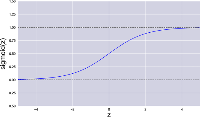
Consider what happens if one of the weights in w₁ is very large—either positive or negative. In that case, the sigmoid gets a large input. With a large input, the sigmoid becomes a very flat function, with a gradient close to 0. In technical terms, the sigmoid gets saturated: it’s pushed outside of its ideal range of operation, to a place where its gradient becomes tiny.
During backpropagation, that tiny gradient gets multiplied by all the other gradients in the chain, resulting in a small overall gradient. In turn, that small gradient forces gradient descent to take very tiny steps.
To summarize this dismaying chain of cause and effect: the larger the weight, the flatter the sigmoid; the flatter the sigmoid, the smaller the gradient; the smaller the gradient, the slower GD; and the slower GD, the less the weight changes. A handful of large weights are enough to slow the entire training to a crawl.
If the numbers in the network get even larger, things go south fast. Imagine that the network has an input with a value of 10, and a weight that’s around 1000. See what happens when those weight and input are multiplied and fed to the sigmoid:
| => | import neural_network as nn |
| => | weighted_sum = 1000 * 10 |
| => | nn.sigmoid(weighted_sum) |
| <= | 1.0 |
The sigmoid saturated: it got so close to 1, that it underflowed and just returned 1. Even worse, its gradient underflowed to 0:
| => | nn.sigmoid_gradient(nn.sigmoid(weighted_sum)) |
| <= | 0.0 |
Remember the chain rule? During backpropagation, this gradient of 0 gets multiplied by the other local gradients, causing the entire gradient to become 0. With a gradient of 0, gradient descent has nowhere to go. This weight is never going to change again, no matter how long we train the network. In machine learning lingo, the node associated with this weight has become a dead neuron.
In the first page of this chapter, I mentioned that backpropagation comes with a few subtle consequences. Dead neurons are one of them. A dead neuron is stuck to the same value forever. It never learns, and doesn’t contribute to GD. If too many neurons die, the network loses power—and worse, you might not even notice.
So, how do we prevent dead neurons?
Weight Initialization Done Right
Let’s wrap up what we said in the previous sections. We should initialize weights with values that are:
- Random (to break symmetry)
- Small (to speed up training and avoid dead neurons)
It’s hard to gauge how small exactly the weights should be. In Part III of this book, we’ll look at a few popular formulae to initialize weights. For now, we can use an empirical rule of thumb. We’ll make each weight range from 0 to something around the following value, where r is the number of rows in the weight matrix:
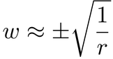
Read it as: the absolute value of each weight shouldn’t be much bigger than the square root of the inverse of rows. That idea makes more sense if you think that all weights add something to the network’s output—so, as the weight matrix gets bigger, individual weights should become smaller.
Here is a function that initializes the weights with the previous formula:
| | def initialize_weights(n_input_variables, n_hidden_nodes, n_classes): |
| | w1_rows = n_input_variables + 1 |
| | w1 = np.random.randn(w1_rows, n_hidden_nodes) * np.sqrt(1 / w1_rows) |
| | |
| | w2_rows = n_hidden_nodes + 1 |
| | w2 = np.random.randn(w2_rows, n_classes) * np.sqrt(1 / w2_rows) |
| | |
| | return (w1, w2) |
NumPy’s random.randn function returns a matrix of random numbers taken from what is called the standard normal distribution. In practice, that means that the random numbers are small: they might be positive or negative, but unlikely to stray far from 0. The code creates two such matrices of weights, and then scales them by the range suggested by our rule-of-thumb formula.
Math Deep Dive: The Standard Normal Distribution | |
|---|---|

|
You might be curious about the standard normal distribution. What does it look like, and why does it generate numbers that are close to zero? To wrap your mind around it, check out Khan Academy’s lessons on modeling data distributions.[19] |
If you’re confused by the dimensions of the two matrices, remember the rule that we mentioned in How Many Nodes?: each matrix of weights in a neural network has as many rows as its input elements, and as many columns as its output elements.
Did you hear that “click” sound? That was the last piece of our neural network’s code falling into place. We’re finally about to run this thing!