Building a Neural Network with Keras
Python boasts a few large ML libraries such as PyTorch[23] and TensorFlow.[24] They’re complex, and they tend to evolve fast. I won’t use them in this book, or even talk about them. If I did, my code examples and explanations would likely be obsolete by the time you read these pages.
Instead, I’ll use a slimmer and more stable library named Keras.[25] Keras is a thin layer that sits on top of the “big” libraries and hides them behind a nice, clean programming interface. Keras started out as a tool for prototyping, but it quickly became one of the most popular ways to build neural networks in Python—it was even adopted by TensorFlow as an official interface. With Keras, we can use the heavyweight libraries without getting bogged down by their complexities.
There are different ways to install Keras, depending on your operating system, your CPU and GPU, and so on. On most systems, you can install it like other libraries: either globally via pip, or inside a Conda environment. To install globally:
| | pip3 install keras |
Alternatively, here’s how you install Keras in the machinelearning Conda environment:
| | conda activate machinelearning |
| | conda install keras |
When you install Keras, you also get TensorFlow—so you can start building neural networks straight away.
A Plan and a Piece of Code
Let’s build a neural network for the Echidna dataset. As a starting point, we can use the MNIST network that we designed back in Chapter 9, Designing the Network. Here it is:
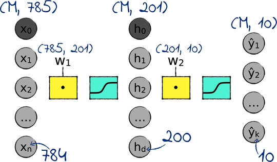
As a reminder, M is the number of examples in the training set, and 784 is the number of input variables in MNIST. Here is how we can modify this network to learn the Echidna dataset instead:
-
The Echidna dataset has two input variables, so we only need two input nodes.
-
The Echidna dataset has two classes, so we only need two output nodes instead of 10.
-
The number of hidden nodes is a hyperparameter that we can change later. To begin with, let’s go with 100 hidden nodes.
-
Finally, the MNIST network is complicated by the bias nodes x₀ and h₀. We have good news here: Keras takes care of the bias under the hood, so we can forget about the bias nodes altogether.
After applying those changes, here is the plan for our new network:
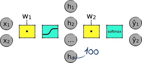
Now I’m going to show you how you can implement this network with Keras. I’m about to drop the entire neural network code right in your lap. Don’t worry if it looks confusing—we’ll step through it in a minute. Here is the whole thing:
| | from keras.models import Sequential |
| | from keras.layers import Dense |
| | from keras.optimizers import RMSprop |
| | from keras.utils import to_categorical |
| | import echidna as data |
| | |
| | X_train = data.X_train |
| | X_validation = data.X_validation |
| | Y_train = to_categorical(data.Y_train) |
| | Y_validation = to_categorical(data.Y_validation) |
| | |
| | model = Sequential() |
| | model.add(Dense(100, activation='sigmoid')) |
| | model.add(Dense(2, activation='softmax')) |
| | |
| | model.compile(loss='categorical_crossentropy', |
| | optimizer=RMSprop(lr=0.001), |
| | metrics=['accuracy']) |
| | |
| | model.fit(X_train, Y_train, |
| | validation_data=(X_validation, Y_validation), |
| | epochs=30000, batch_size=25) |
| | |
| | boundary.show(model, data.X_train, data.Y_train) |
That isn’t much code, considering it’s building the network, training it, and even checking its accuracy on the validation set. Let’s step through this program line by line.
Loading the Data
The first few lines in the Keras neural network focus on preparing the training set and the validation set:
| | from keras.utils import to_categorical |
| | import echidna as data |
| | |
| | X_train = data.X_train |
| | X_validation = data.X_validation |
| | Y_train = to_categorical(data.Y_train) |
| | Y_validation = to_categorical(data.Y_validation) |
X_train and X_validation are the same as in echidna.py—the previous code just renames them for consistency. On the other hand, the labels require some more processing because echidna.py doesn’t one-hot encode them. The last two lines one-hot encode the labels with Keras’s to_categorical function, which behaves the same as the one_hot_encode function we wrote ourselves in Part I. In other words, to_categorical converts the labels from this…
| => | data.Y_train[0:3] |
| <= | array([[0], |
| | [1], |
| | [1]]) |
…to this:
| => | to_categorical(data.Y_train[0:3]) |
| <= | array([[1., 0.], |
| | [0., 1.], |
| | [0., 1.]], dtype=float32) |
The data is in—now let’s assemble the network.
Creating the Model
The next few lines define the shape of the neural network:
| | model = Sequential() |
| | model.add(Dense(100, activation='sigmoid')) |
| | model.add(Dense(2, activation='softmax')) |
This code uses the object-oriented features of Python. (If you know nothing about objects and classes, then maybe read Creating and Using Objects to get up to speed. It will only take you a few minutes.)
The first line in the code creates a “sequential model,” so called because it assembles a neural network as a sequence of layers. Keras comes with a few options for building a neural network, but in this book we’ll always use the sequential model.
The second and third line create the hidden layer and the output layer, and add them to the network. There is no need to create an input layer, because Keras takes care of that automatically: as soon as we start feeding data to the network, Keras will look at the shape of the data and create an input layer with a matching number of nodes, which in our case is two. As I mentioned earlier, Keras will also add a bias node to the input and the hidden layer, so we don’t need to worry about the bias either.
The model and the layers are Python objects: the model is an object of class Sequential, and the layers are objects of class Dense. A layer is dense when each of its nodes is connected to all the nodes in a neighboring layer. We’ll look at other types of layers in the next chapters. For the time being, dense layers will be the only layers we deal with.
To create a Dense layer, Keras needs two arguments: the number of nodes, and the name of an activation function. Keras supports all the popular activation functions, including the two that we need in this network: the sigmoid and the softmax. Note that for each layer, we specify the activation function that comes before the layer, not after it.
We have a neural network. That was quick! Now let’s configure it.
Compiling the Model
The next statement configures the neural network—or, in the lingo of Keras, “compiles” it:
| | model.compile(loss='categorical_crossentropy', |
| | optimizer=RMSprop(lr=0.001), |
| | metrics=['accuracy']) |
First, this statement tells Keras which formula to use for the loss. We want the same formula we used for the MNIST network in Part II: the cross-entropy loss, which Keras calls categorical_crossentropy.
Second, this statement tells Keras which algorithm it should use to minimize the loss during training. Keras comes with multiple flavors of gradient descent—in fact, I cheated a bit here: instead of plain vanilla GD (which Keras calls SGD), this code uses a souped-up version of GD called RMSprop. RMSprop is generally better and faster than SGD, and that extra speed will be welcome when we start experimenting with this network. I’ll go into the details of RMSprop in Chapter 18, Making It Better.
When we create the RMSprop object, we also pass it the parameters that this particular algorithm needs. RMSprop only needs one parameter: the learning rate lr.
Finally, the last parameter to compile tells Keras which metrics to report during training. By default, Keras only prints one metric on the terminal: the loss. In this case, we tell it that we also want to track the accuracy.
Networking configuration: check. Let’s move on to the training phase.
Training the Network
The next statement trains the network—or “fits” it, as Keras prefers to say:
| | model.fit(X_train, Y_train, |
| | validation_data=(X_validation, Y_validation), |
| | epochs=30000, batch_size=25) |
Besides the training set, fit takes an optional parameter with the validation set. If you pass it the validation set, as in the previous code, Keras will print out your validation loss and accuracy at the end of each epoch, together with the training loss and accuracy. The call to fit is also where we specify the remaining two hyperparameters: epochs and batch_size.
We’re almost done with the neural network’s code. We just have one last line to go through.
Drawing the Boundary
The last line in the program prints out the neural network’s decision boundary. That’s not a Keras feature—it’s a little utility I wrote called boundary.py that you can find in this chapter’s source code. The boundary.show function takes a trained neural network and a bi-dimensional dataset, and prints out the network’s decision boundary over the dataset:
| | import boundary |
| | |
| | boundary.show(model, data.X_train, data.Y_train) |
Note that boundary.show takes the labels without one-hot encoding.
With that, we have all it takes to run this neural network on the Echidna dataset, measure its accuracy on the training and the validation set, and check out its decision boundary. Let’s run this thing!
Keras in Action
Training the neural network took me a few minutes on my laptop. Here’s the output, stripped down to the essential information:
| | Using TensorFlow backend. |
| | Train on 285 samples, validate on 285 samples |
| | Epoch 1 - loss: 0.7222 - acc: 0.5088 - val_loss: 0.6928 - val_acc: 0.4807 |
| | Epoch 2 - loss: 0.6966 - acc: 0.5018 - val_loss: 0.6904 - val_acc: 0.5193 |
| | … |
| | Epoch 30000 - loss: 0.1623 - acc: 0.9193 - val_loss: 0.1975 - val_acc: 0.9018 |
The accuracy on the training set gets up to 0.9193—that is, 91.93%. However, we know from Training vs. Testing that the training accuracy could be polluted by overfitting. Instead, we should look at the validation accuracy: 90.18%.
Now let’s check out the network’s decision boundary:
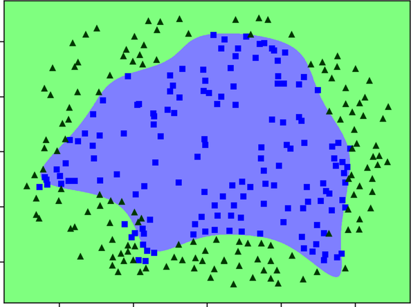
The network did a decent job of finding a boundary that separates the data points inside and outside the echidna shape. However, it doesn’t seem very good at contouring small details like the echidna’s nose and claws. That lack of finesse in the boundary explains why the neural network misclassifies about one point in ten.
Maybe a deeper network might do better on those small details? After all, that’s the selling point of deep learning: just like a shallow neural network tracks the twists in a dataset better than a perceptron, a deep neural network should do even better.
Let’s find out for ourselves, by adding a layer to our neural network.