Adding More Tricks to Your Bag
Picking the right activation functions is a crucial decision, but when you design a neural network, you face plenty more. You decide how to initialize the weights, which GD algorithm to use, what kind of regularization to apply, and so forth. You have a wide range of techniques to choose from, and new ones come up all the time.
It would be pointless to go into too much detail about all the popular techniques available today. You could fill entire volumes with them. Besides, some of them might be old-fashioned and quaint by the time you read this book.
For those reasons, this section doesn’t aspire to be comprehensive. See it like a quick shopping spree in the mall of modern neural networks: we’ll look at a handful of techniques that generally work well—a starter’s kit in your journey to ML mastery. At the end of this chapter, you’ll also get a chance to test these techniques first hand.
Let’s start with weight initialization.
Better Weight Initialization
You learned a few things about initializing weights in Initializing the Weights. In case you don’t remember that section, here’s the one-sentence summary: to avoid squandering a neural network’s power, initialize its weights with values that are random and small.
That “random and small” principle, however, doesn’t give you concrete numbers. For that, you can use a formula such as Xavier initialization, also known as Glorot initialization. (Both names come from Xavier Glorot, the dude who proposed it.)
Xavier initialization comes in a few variants. They all give you an approximate range to initialize the weights, based on the number of nodes connected to them. One common variant gives you this this range:
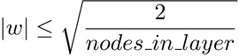
The core concept of Xavier initialization is that the more nodes you have in a layer, the smaller the weights. Intuitively, that means that it doesn’t matter how many nodes you have in a layer—the weighted sum of the nodes stays about the same size. Without Xavier initialization, a layer with many nodes would generate a large weighted sum, and that large number could cause problems like dead neurons and vanishing or exploding gradients.
Even though I didn’t mention Xavier initialization so far, we already used it: it’s the default initializer in Keras. If you want to replace it with another initialization method, of which Keras has a few, use the kernel_initializer argument. For example, here is a layer that uses an alternative weight initialization method called He normal:
| | model.add(Dense(100, kernel_initializer='he_normal')) |
Gradient Descent on Steroids
If something stayed unchanged through this book, it’s the gradient descent algorithm. We changed the way we compute that gradient, from simple derivatives to backpropagation, but so far, the “descent” part is the same as I introduced it in the first chapters: multiply the gradient by the learning rate and take a step in the opposite direction.
Modern GD, however, can be subtler than that. In Keras, you can pass additional parameters to the SGD algorithm:
| | model.compile(loss='categorical_crossentropy', |
| » | optimizer=SGD(lr=0.1, decay=1e-6, momentum=0.9), |
| | metrics=['accuracy']) |
This code includes two new hyperparameters that tweak SGD. To understand decay, remember that the learning rate is a trade-off: the smaller it is, the smaller each steps of GD—that makes the algorithm more precise, but also slower. When you use decay, the learning rate decreases a bit at each step. A well-configured decay causes GD to take big leaps in the beginning of training, when you usually need speed, and baby steps near the end, when you’d rather have precision. This twist on GD is called learning rate decay, that’s a refreshingly descriptive name.
The momentum hyperparameter is even subtler. When I introduced GD, you learned that this algorithm has trouble with certain surfaces. For example, it might get stuck into local minima—that is, “holes” in the loss. Another troublesome situation can happen around “canyons” like the one shown in the following diagram:
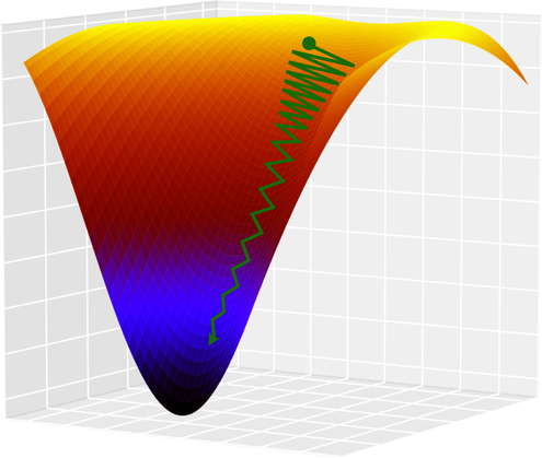
GD always moves downhill in the direction of the steeper gradient. In the upper part of this surface, the walls of the canyon are steeper than the path toward the minimum—so GD ends up bouncing back and forth between those walls, barely moving toward the minimum at all.
For this example, I drew a hypothetical path on a three-dimensional surface. However, cases such as this one are common in real life on higher-dimensional loss surfaces. When they happen, the loss might stop decreasing for many epochs in a row, leading you to believe that GD has reached a minimum, and giving up on training.
That’s where the momentum algorithm enters the scene. That algorithm counters the situation I just described by adding an “acceleration” component to GD. That makes for a smoother, less jagged path, as shown in the diagram.

Momentum can speed up training tremendously. In some cases, it may even help GD zip over local minima, propelling it toward the lowest loss. The result is not only faster training, but also higher accuracy.
In Keras, decay and momentum are additional parameters to the standard SGD algorithm. However, Keras also comes with entirely different implementations of GD, which it calls “optimizers.” One of those alternatives to SGD is the RMSprop optimizer, that implements a concept similar to momentum. I already sneakily used RMSprop when I wrote our first deep network in Chapter 16, A Deeper Kind of Network. It made the network’s training radically faster and more efficient than SGD:
| | model.compile(loss='categorical_crossentropy', |
| » | optimizer=RMSprop(lr=0.001), |
| | metrics=['accuracy']) |
That’s all I wanted to tell you about optimizers. If you want to do some research on your own, another optimizer worth checking out is called Adam. It’s very popular these days, and it merges momentum and RMSprop into one mean algorithm.
Advanced Regularization
When it comes to overfitting, deep neural networks need all the help they can get. In the previous chapter you learned about the classic L1 and L2 regularization techniques. However, more modern techniques often work better. One in particular, called dropout, is very effective—and also somewhat weird.
Dropout is based on a striking premise: you can reduce overfitting by randomly turning off some nodes in the network. You can see dropout as a filter attached to a layer that randomly disconnects some nodes during each iteration, as illustrated by the following diagram:
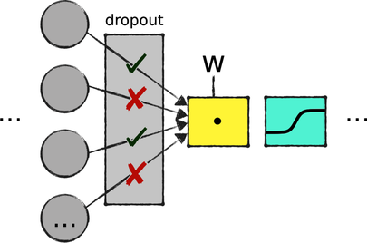
Disconnected nodes don’t impact the next layers, and they’re ignored by backpropagation. It’s like they cease to exist until the next iteration.
To use dropout in Keras, you add Dropout layers on top of regular hidden layers. You can specify the fraction of nodes to turn off at each iteration—in this example, 25%:
| | from keras.layers import Dropout |
| | |
| | model = Sequential() |
| | model.add(Dense(500, activation='sigmoid')) |
| | model.add(Dropout(0.25)) |
| | model.add(Dense(200, activation='sigmoid')) |
| | model.add(Dropout(0.25)) |
| | model.add(Dense(10, activation='softmax')) |
I’ve just described how dropout works—but not why it works. It’s kinda hard to understand intuitively why dropout reduces overfitting, but here’s a shot at it: dropout forces the network to learn in a slightly different way at each iteration of training. In a sense, dropout reshapes one big network into many smaller networks, each of which might learn a different facet of the data. Where a big network is prone to memorize the training set, each small network ends up learning the data its own way, and their combined knowledge is less likely to overfit the data.
That’s only one of a few possible ways to explain the effect of dropout. Whatever our intuitive understanding, however, dropout works—and that’s what counts. It’s one of the first regularization techniques I reach for in the presence of overfitting.
Speaking about things that work, although it’s hard to see why: there is one last technique I want to tell you about in this chapter.
One Last Trick: Batch Normalization
Think back to the idea of standardizing data, which we looked at in Preparing Data. In a sentence, a standardized dataset is centered on zero and doesn’t stray far from there. As I explained when I introduced this topic, neural networks like small, zero-centered numbers.
Standardization, however, can only go so far. As our carefully standardized data moves through the network, it changes, losing its network-friendly shape. It would be nice if each hidden layer received standardized inputs, not just the input layer. That’s pretty much what batch normalization does: it re-standardizes each batch of data before it enters each network layer.
Batch normalization involves a few technical complexities. For one, it doesn’t necessarily use an average of 0 and a standard deviation of 1, like regular input standardization. Instead, its average and standard deviation are themselves learnable parameters that are tuned by gradient descent. However, you can leave those technical details to Keras and use batch normalization as a black box:
| | from keras.layers import BatchNormalization |
| | |
| | model = Sequential() |
| | model.add(Dense(500, activation='sigmoid')) |
| | model.add(BatchNormalization()) |
| | model.add(Dense(200, activation='sigmoid')) |
| | model.add(BatchNormalization()) |
| | model.add(Dense(10, activation='softmax')) |
When it was introduced (around 2015), batch normalization was hailed as a breakthrough. You might say that it’s an advanced technique—but even beginners are keen to use it because it works so darn well. It often improves a network’s accuracy, and sometimes even speeds up training and reduces overfitting. There is no such thing as an easy win in deep learning, but batch normalization comes as close as anything.