1. Introduction
In this introductory chapter a short MATLAB tutorial is provided. This tutorial describes the basic MATLAB commands needed. More details about these commands will follow in subsequent chapters. Note that there are numerous free MATLAB tutorials on the internet – check references [1-28]. Also, you may want to consult many of the excellent books on the subject – check references [29-47]. This chapter may be skipped on a first reading of the book.
In this tutorial it is assumed that you have started MATLAB on your computer system successfully and that you are now ready to type the commands at the MATLAB prompt (which is denoted by double arrows “>>”). For installing MATLAB on your computer system, check the web links provided at the end of the book.
Entering scalars and simple operations is easy as is shown in the examples below:
>> 2*3+5
ans =
11
The order of the operations will be discussed in subsequent chapters.
>> cos(60*pi/180)
ans =
0.5000
The argument for the cos command and the value of pi will be discussed in subsequent chapters.
We assign the value of 4 to the variable x as follows:
>> x = 4
x =
4
>> 3/sqrt(2+x)
ans =
1.2247
To suppress the output in MATLAB use a semicolon to end the command line as in the following examples. If the semicolon is not used then the output will be shown by MATLAB:
>> y = 30;
>> z = 8;
>> x = 2; y-z;
>> w = 4*y + 3*z
w =
144
MATLAB is case-sensitive, i.e. variables with lowercase letters are different than variables with uppercase letters. Consider the following examples using the variables x and X:
Use the help command to obtain help on any particular MATLAB command. The following example demonstrates the use of help to obtain help on the det command which calculated the determinant of a matrix:
>> help det
DET Determinant.
DET(X) is the determinant of the square matrix X.
Use COND instead of DET to test for matrix singularity.
See also cond.
Overloaded functions or methods (ones with the same name in other directories)
help sym/det.m
Reference page in Help browser doc det
The following examples show how to enter matrices and perform some simple matrix operations:
>> x = [1 2 3 ; 4 5 6 ; 7 8 9]
x =
1 2 3
4 5 6
7 8 9
>> y = [1 ; 0 ; -4]
y =
1
0
-4
>> w = x*y
w =
-11
-20
-29
Let us now see how to use MATLAB to solve a system of simultaneous algebraic equations. Let us solve the following system of simultaneous algebraic equations:

We will use Gaussian elimination to solve the above system of equations. This is performed in MATLAB by using the backslash operator “\” as follows:
>> A= [3 5 -1 ; 0 4 2 ; -2 1 5]
A =
3 5 -1
0 4 2
-2 1 5
>> b = [2 ; 1 ; -4]
b =
2
1
-4
>> x = A\b
x =
-1.7692
1.1154
-1.7308
It is clear that the solution is x1 = -1.7692, x2 = 1.1154, and x3 = -1.7308. Alternatively, one can use the inverse matrix of A to obtain the same solution directly as follows:
>> x = inv(A)*b
x =
-1.7692
1.1154
-1.7308
It should be noted that using the inverse method usually takes longer than using Gaussian elimination especially for large systems of equations.
Consider now the following 4 x 4 matrix D:
>> D = [1 2 3 4 ; 2 4 6 8 ; 3 6 9 12 ; -5 -3 -1 0]
D =
1 2 3 4
2 4 6 8
3 6 9 12
-5 -3 -1 0
We can extract the sub-matrix in rows 2 to 4 and columns 1 to 3 as follows:
We can extract the third column of D as follows:
>> F = D(1:4, 3)
F =
3
6
9
-1
We can extract the second row of D as follows:
>> G = D(2, 1:4)
G =
2 4 6 8
We can also extract the element in row 3 and column 2 as follows:
>> H = D(3,2)
H =
6
We will now show how to produce a two-dimensional plot using MATLAB. In order to plot a graph of the function y = f (x) , we use the MATLAB command plot(x,y) after we have adequately defined both vectors x and y. The following is a simple example to plot the function y = x2 + 3 for a certain range:
>> x = [1 2 3 4 5 6 7 8 9 10 11]
x =
Columns 1 through 10
1 2 3 4 5 6 7 8 9 10
Column 11
11
>> y = x.^2 + 3
y =
Columns 1 through 10
4 7 12 19 28 39 52 67 84 103
Column 11
124
>> plot(x,y)
Figure 1.1 shows the plot obtained by MATLAB. It is usually shown in a separate window. In this figure no titles are given to the x- and y-axes. These titles may be easily added to the figure using the xlabel and ylabel commands. More details about these commands will be presented in the chapter on graphs.
In the calculation of the values of the vector y, notice the dot “.” before the exponentiation symbol “^”. This dot is used to denote that the operation following it be performed element by element. More details about this issue will be discussed in subsequent chapters.
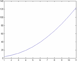
Figure 1.1: Using the MATLAB "plot" command
Finally, we will show how to make magic squares with MATLAB. A magic square is a square grid of numbers where the total of any row, column, or diagonal is the same. Magic squares are produced by MATLAB using the command magic. Here is a simple example to produce a 5 x 5 magic square:
>> magic(5)
ans =
17 24 1 8 15
23 5 7 14 16
4 6 13 20 22
10 12 19 21 3
11 18 25 2 9
It is clear that the total of each row, column or diagonal in the above matrix is 65.
Exercises
Solve all the exercises using MATLAB. All the needed MATLAB commands for these exercises were presented in this chapter.
- Perform the operation 3*4+6. The order of the operations will be discussed in subsequent chapters.
- Perform the operation cos(5) . The value of
5is in radians. - Perform the operation
 for x = 4 .
 - Assign the value of 5.2 to the variable
y. - Assign the values of 3 and 4 to the variables
xandy, respectively, then calculate the value ofzwhere z = 2x − 7 y . - Obtain help on the
invcommand. - Generate the following matrix:
A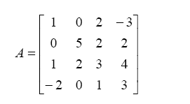
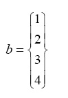
- Generate the following vector
b - Evaluate the vector
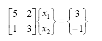
cwhere {c} = [A]{b} whereAis the matrix given in Exercise 7 above andbis the vector given in Exercise 8 above. - Solve the following system of simultaneous algebraic equation using Gaussian elimination.
- Solve the system of simultaneous algebraic equations of Exercise 10 above using matrix inversion.
- Generate the following matrix
X: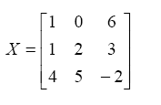
- Extract the sub-matrix in rows 2 to 3 and columns 1 to 2 of the matrix
Xin Exercise 12 above. - Extract the second column of the matrix
Xin Exercise 12 above. - Extract the first row of the matrix
Xin Exercise 12 above. - Extract the element in row 1 and column 3 of the matrix
Xin Exercise 12 above. - Generate the row vector
xwith integer values ranging from 1 to 9. - Plot the graph of the function y = x3 − 2 for the range of the values of
xin Exercise 17 above. - Generate a 4 x 4 magic square. What is the total of each row, column, and diagonal in this matrix.