TABLE 19.1 Prisoner’s Dilemma
There exists everywhere a medium in things,
determined by equilibrium.
—DMITRI MENDELEEV
First, let’s look at what is known as a normal form description of a game. Normal form games are good places to start because they are rather simple. In this form, you represent the game as a table or matrix. One player’s options are presented by the matrix’s rows. The other player (given a two-player game) has options represented by the columns of the matrix. Where each intersects is the result of the game with each player receiving a payoff.
Where game theory is useful is in determining not what a player can do, but what a player will do. You need to make a bunch of assumptions in order to determine this, but it can help you to determine whether any options in your game are not logical to ever choose. The result in which players are theorized to end up is the equilibrium result.
Equilibria tell us what behaviors are likely to emerge from a particular set of rules.
The classic example that is always the introduction to game theory anywhere it is taught is called the Prisoner’s Dilemma. It is set up thusly:
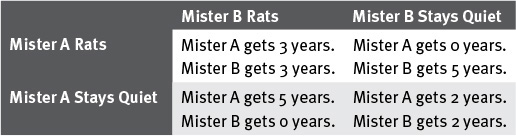
Mister A and Mister B have been apprehended on suspicion of a robbery. Both are isolated and have no opportunity to communicate with each other. The police can already get them both for criminal trespassing and conspiracy, which will result in a two-year sentence. The police give the two the same choice. Become an informant and rat on the partner. In this case, the “rat” would have his charges dropped and the other criminal would get five years in prison for the robbery, criminal trespassing, and conspiracy. However, if both rat, then they will both receive the robbery charge of three years.
What should Mister A and Mister B do? Game theory considers this a game: It has players (Mister A and Mister B), actions (rat or stay quiet), information, and payoffs (sentences). This type of game is usually examined using a table, as in TABLE 19.1.
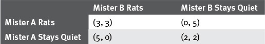
The payoff cells (sentences) are a bit wordy and redundant, so payoffs are usually listed as a tuple with the payoffs for each player, as shown in TABLE 19.2. The sentences are given as (Mister A’s sentence in years, Mister B’s sentence in years).
How can someone predict what Mister A and Mister B will do? First, they assume that both criminals are rational, that both understand all the payoffs in the game, and that both players will try to minimize their individual sentences. No weight is given to any loyalty or possible repercussions outside the game. The players are selfish and all rewards are built into the listed payoffs.
Look at Table 19.2 from Mister A’s perspective; this shows that ratting is always preferable to staying quiet, no matter what Mister B does. If Mister B rats, then by ratting, Mister A gets three years instead of five. If Mister B stays quiet, then by ratting, Mister A gets zero years instead of two. Either way ratting is better for Mister A.
But this game is symmetric. Mister B’s incentives are the same as Mister A’s. From Mister B’s perspective, his results are also always better if he rats. Thus, both should rat.
This is interesting because by acting in their own best interests, they get a worse result than if they cooperate. By following the best strategy, both serve three years, whereas by cooperating, they would have each only served two. The (2,2) result is known as Pareto optimal. It is a result where no one can become better off without making someone else worse off.
However, the (3,3) result is the equilibrium result. It is the result for which changing a decision in isolation (and with all other players knowing about the switch) would result in a worse outcome for the player choosing to switch.
In game theory terms, you say that “rat” strictly dominates “stay quiet” for both players. No matter what the other player chooses, choosing “rat” gives the player a better outcome than choosing “stay quiet.” To be strictly dominant, a strategy must produce a better result than any other strategy no matter what an opponent does. Any option that is dominated cannot be equilibrium. If an option is dominated, it means that something else is always better, so why would the players ever pick it?
A game where the equilibrium is also Pareto optimal is called deadlock. In deadlock, both players end on an outcome that is mutually beneficial. It is essentially identical to the Prisoner’s Dilemma except that the Pareto optimal result is also the equilibrium.
If you wish to know what the players should do, you must solve for the game’s equilibria. When you first look at a matrix of payoffs, any outcome could be an equilibrium outcome. Most games are not as easy to solve as the Prisoner’s Dilemma. You can use several techniques to best eliminate results to find the true equilibria. One technique is known as Iterated Elimination of Dominated Strategies. That is a mouthful for a way of doing something similar to what we did to solve the Prisoner’s Dilemma in the previous section.
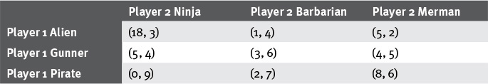
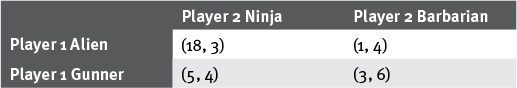
Imagine a game, explained by TABLE 19.3, in which two players have to choose a character and then each gets points based on how well those characters perform against each other. You can read the table data as “number of points for player 1, number of points for player 2.” Which player has the advantage?
A naive strategy would be to take the average points for each player. Here each player has an average result of 5.11 points, so an (incorrect) answer would be that neither player has the advantage.
If you assume that players know all this information, and if players act rationally in their own best interests (all assumptions made in game theory), then you can predict what will happen in this game. You can eliminate any options that are strictly dominated by another option. Remember that an Option A that has strict dominance over Option B means that Option A is better than Option B under every circumstance. If Option A is equal to Option B at any point, this analysis will not necessarily work.
In examining strict dominance, you focus only on one player’s perspective at a time. It can often be helpful to remove the other player’s payoffs because they can be a distraction. If the player is only trying to maximize his own score, he will not care what score the opponent receives. (A zero-sum game where one player’s “plus one” is another player’s “minus one” would be different).
Looking from Player 2’s perspective, remove the option of Ninja temporarily and look only at the decision between Barbarian and Merman in TABLE 19.4.
 Note
Note
The choice to remove the Ninja option and examine the remaining two options doesn’t have any science behind it. You may choose any two options to examine, but these two are worth examining because one ends up strictly dominating the other. That will not always be the case. You may need to try many different combinations before finding a pair that shows strict dominance.
The points for choosing Barbarian are always greater than the points for choosing Merman. Thus, both players should know that Player 2 will never choose Merman as long as that player can choose Barbarian. It doesn’t matter if you add Ninja back in. If Ninja is better than Merman, that player will not pick Merman. If Ninja is worse than Merman, that player will not pick Merman; as you know, he will pick Barbarian. Now that you know that Merman will not be chosen as long as Barbarian is an option, you can remove it from the game permanently. Bring Ninja back; you were just isolating it for a moment.
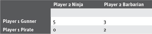
This opens a new layer to the analysis. Now that Pirate-Merman has been deleted, there is a dominant relationship between Pirate and Gunner for Player 1. Remove Alien temporarily and look at only Gunner versus Pirate in terms of Player 1’s points (TABLE 19.5). Remember that the choice between Gunner and Pirate belongs to Player 1, so consider only the payoffs for Player 1. As you can see, Gunner is always preferable to Pirate.
This narrows the game further because now you know that Pirate will never be chosen by Player 1, so you can remove it permanently.
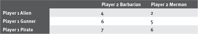
You are left with two options for each player. For Player 1, neither Alien nor Gunner is dominant (TABLE 19.6). However, looking from Player 2’s perspective, Barbarian is always better than Ninja. (4 versus 3 if Player 1 chooses Alien and 6 versus 4 if Player 1 chooses Gunner). This means you know that Player 2 should choose Barbarian.
You now have a pretty simple game to solve (TABLE 19.7). Since 3 is better than 1, Player 1 will choose Gunner over Alien. The equilibrium is that Player 1 should choose Gunner and Player 2 should choose Barbarian. The equilibrium result is (3, 6), thus Player 2 has the advantage.
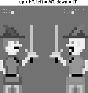
By eliminating dominated options in your games, you are left with only the options that players can weigh for interesting decisions. If a player can reduce a game down to a single pure strategy, then what interesting decision is left? The game submission, shown in FIGURE 19.1, that I received in a game design class illustrates this point well.
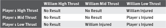
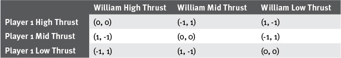
It was a swordfighting game where the player simultaneously acted with the AI opponent by pressing one of the arrow keys to choose “high thrust,” “mid thrust,” or “low thrust.” The result would either injure you (Player 1, on the right), injure your opponent (William, in the dashing purple smock to the left), or have no result. After digging through the student’s code, I was able to deduce the results in TABLE 19.8.
A cursory glance at this would lead you to say, “There are two scenarios in which William is injured and two scenarios in which Player 1 is injured. This must be fair.” But look closer; you’ll see the problem. What is Player 1 incentivized to choose? If he chooses high thrust, the possible outcomes are a draw or a point against the opponent. Player 1 can’t lose if he chooses high thrust! At worst, he can tie. Now look at if Player 1 chooses mid thrust. The possible outcomes are a draw or a point against the player! Nothing good comes out of choosing mid thrust. Player 1 can never win when choosing this. Low thrust is the most interesting because the player can hit the opponent or the opponent can hit the player. But why would he ever choose that when he has the safety of high thrust?
The student creator of this game chose to code William so that he picked each of the thrusts one-third of the time randomly. But if William was an actual rational human player, what would he do? Mid thrust is as bad for him as it is for the Player 1. High thrust is always a draw for him. Low thrust allows him to score a point as long as the opponent does not pick high thrust, so at first it seems the best choice. But if you assume William knows the rules of the game, he knows that Player 1 will pick high thrust, so he is incentivized to pick high thrust as well. (If he picked mid thrust and Player 1 knew that he would pick mid thrust, Player 1 could always switch to low thrust and score a point, so William has no incentive to ever pick mid thrust). As a result, if both players are playing rationally, they both always pick high thrust against each other and the game is a perpetual draw. Boring, right?
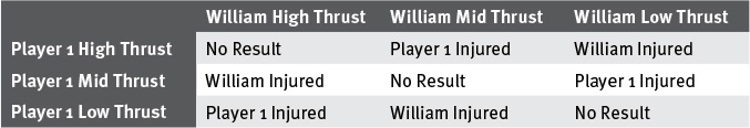
How can you fix this? You need to remove the domination from each player’s options. Look at TABLE 19.9, where I’ve made sure that each thrust has one win state, one lose state, and one draw for each player.
Or take a look at TABLE 19.10, which uses numbers for the data.
With these results, both players are not incentivized to favor any particular technique. The mixed equilibrium is at  for each type of attack. But does it look familiar?
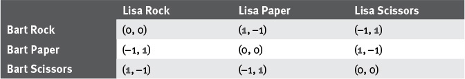
Rock, Paper, Scissors (TABLE 19.11) interests game designers because it is an extremely simple game whose only equilibrium is in mixed strategies—throwing one move some times and changing it up often. It does not make for informed choice (since every strategy is as good as any other), but it is certainly better than pure, dominated strategies. In game theory, this “A beats B, B bests C, C beats A” system is known as intransitive. Many popular games use intransitive systems as a base, such as Pokemon.
If a game’s key decisions end up being dominated, some of its options are never played. Not only is this boring from a play perspective, but it means the creators are going to have to create code and assets for situations that should never come up, which is wasted effort. A better design looks for equilibrium only in mixed strategies in which each option has a probability greater than zero of being chosen. This ensures that all options have an opportunity to be played, and the resulting system is more interesting.
Head-to-head games are often zero-sum games. In a zero-sum game, the amount of resources stays the same for all players. For example, a game in which I flip a coin, you give me $20 if it lands Heads, and I give you $5 if it lands Tails is a zero-sum game. Even though it is unfair to you, no matter what happens, the amount of money between us stays the same; we are only transferring resources. Rock, Paper, Scissors is a zero-sum game; if a player wins, the opponent loses.
In all two-player zero-sum games, a strategy known as minimax solves the game. In minimax, each player forms a strategy that minimizes the pain of their worst-case scenario. In the first “William versus the Player” swordfighting example in Table 19.8, the minimal pain for Player 1 is to choose high thrust. Mid thrust and low thrust each have a worst-case scenario of injury. High thrust’s worst case is no result. William’s worst-case scenario is no result if he chooses high thrust, but injury if he chooses either of the other two attacks. Thus, the minimax solution is for William to high thrust and Player 1 to high thrust—just what you found earlier. This technique works for all two player zero-sum games.
Since this solution is easily findable by players, most interesting games are either not entirely zero-sum, or they become more interesting when a third player (or more) is added to the game.
As a designer, you can use dominance to guide players away from options that you don’t want them to choose. However, the most interesting game decisions often come from solutions with mixed strategies.
The Prisoner’s Dilemma is easy to understand because of its strict dominance. Neither player has to worry about what the other does because there is a better option in all cases. However, in practical application, this is not often the case. Consider this classic example adapted liberally from 18TH Century French philosopher Jean Jacques Rousseau named “The Stag Hunt.”1
1 Rousseau, J. J. (1755). A Discourse on the Origins and Foundations of Inequality Among Men. Trans. Maurice Cranston (1984) Harmondsworth: Penguin.
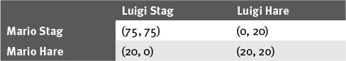
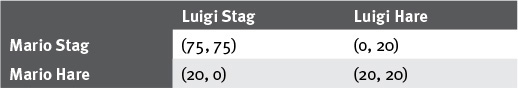
Two hunters (Mario and Luigi) go out to hunt. Each must choose to hunt a stag (a deer) or a hare, and each must choose without knowing what the other hunter chose. If a hunter chooses the stag, he must have the cooperation of his partner to capture the beast. The stag produces 150 lbs of meat. A day’s hunt of hare can produce 20 lbs of meat.
The game can be drawn up as in TABLE 19.12, similar to The Prisoner’s Dilemma.
Examine the game from Mario’s perspective. All else being equal, the best result for him is if he chooses Stag and Luigi chooses Stag as well. But if he chooses Stag and Luigi chooses Hare, he and his family go hungry tonight. Luigi is posed with the same dilemma. If Mario chooses Stag, all is well. But if not, he and his go hungry.
This game doesn’t have strict dominance. No one option is better for one player than any other option, thus you cannot eliminate Stag or Hare for either player.
Another technique for solving this game is to examine each payoff. If neither player can do better by unilaterally changing her strategy holding the other player’s strategy constant, that outcome is a Nash equilibrium.
Look first at (Stag, Stag). Mario would not want to change to Hare since that would lower his payoff. Neither would Luigi. This is a Nash equilibrium. This makes sense as an equilibrium because it is also Pareto optimal. It is the best for everyone. Why would anyone want to change?
Look now at (Stag, Hare). If Luigi knew that Mario chose Stag, he would want to change his strategy to Stag as well, because the 20 he gets from Hare is not as good as the 75 he would get for Stag. Thus, this is not a Nash equilibrium. Since this game is symmetric, the same is true for (Hare, Stag). Mario would change if he knew Luigi chose Stag.
Look finally at (Hare, Hare). If Luigi knew that Mario chose Hare, he certainly wouldn’t change to Stag. That would get him 0 pounds of meat instead of 20. The same is true for Mario. If he knew Luigi chose Hare, then he would not want to switch either. Since neither wants to switch, this is also a Nash equilibrium.
Both players are better off with the (Stag, Stag) equilibrium, but it’s just as rational for players to settle for the (Hare, Hare) equilibrium. If Mario and Luigi ended on (Hare, Hare) or (Stag, Stag), neither has regrets. They chose the best solution given what the other had chosen.
In The Stag Hunt, it is easy to find the Nash equilibria because there are only four possible outcomes. With a more complicated game, it is overly tedious to brute force through every outcome.
In Pokemon, players select creatures that have an inherent “type” to battle each other. In Pokemon X/Y, each attack has one of 18 types, such as Fire, Ground, or Psychic, and each defending Pokemon has a certain inherent type as well. Some types are stronger than others. For instance, a Fire attack is extra effective against an Ice Pokemon, as you would imagine. A Ground attack does not even hit a Flying Pokemon. For 18 Pokemon types and 18 attack types, there is a matrix with 324 outcomes, too tedious to go through one by one.
One technique used to determine Nash equilibria in such cases is to hold each opponent’s selection constant and find what the player’s best choice is. If that outcome ends up being the best choice for all of the players, then it is a Nash equilibrium.
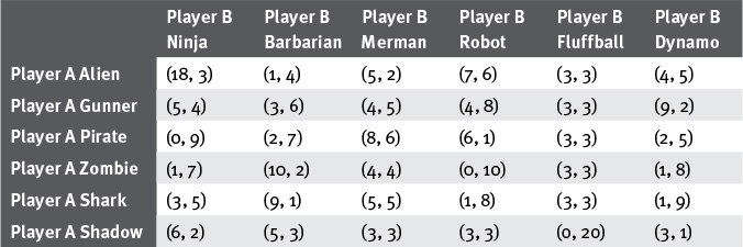
TABLE 19.13 is a matrix that uses the same game from the previous section, eliminating strongly dominated strategies, but it adds a few new types to the mix.
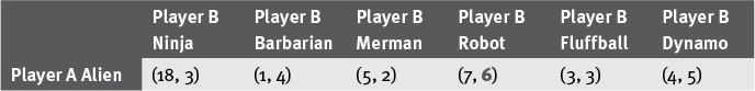
Isolate Player A to choose Alien as in TABLE 19.14. If Player A chooses Alien, then the best bet for Player B is to choose Robot. Indicate Robot for Player B by circling the result, adding an asterisk, or changing the color. Do something that makes that result stand out. Here, if we know Player A chose Alien, Player B’s best bet is to get 6 points by choosing Robot.
Do this for each possible Player A choice. If two choices are equally good, highlight both. For instance, if Player B chooses Fluffball, Player A’s best choice is anything other than Shadow. Highlight all the results except for Shadow. After you have highlighted the best choices for B holding A’s choices constant, hold Player B’s choices constant and find the best option for Player A, highlighting the result for each. After examining all of these, the matrix should look like TABLE 19.15.
There is only one result in this game where both results are highlighted: (Alien, Robot). It is this game’s only Nash equilibrium. If Player A knows that Player B is choosing Robot, then her best choice is to choose Alien because no other option nets her 7 points or more. If Player B knows that Player A is choosing Alien, then choosing Robot is his best choice because it results in 6 points. Neither player has a reason to switch, so this is a Nash equilibrium.
Imagine a game of Rock, Paper, Scissors. You highlight all the best strategies for each player as in TABLE 19.16.
But no result ends up being the best for both players. No pure Nash equilibria exists. This is incredibly common in zero-sum games in which one player directly plays against another, and one’s loss is the other’s gain. Most sports and multiplayer competitive games are organized this way.
How do you actually play Rock, Paper, Scissors? Most of us randomly choose one of the three choices. What if a player weighted one result higher than the others? Say he chose Rock 95 percent of the time. If you knew that, you would play Paper most of the time. If he chose Rock 5 percent of the time and you knew that, you would almost never choose Paper.
Choosing a particular option, no matter what the opponent does, as I have covered before, is known as a pure strategy. It is pure because no matter the situation, the strategy is the same. A mixed strategy involves assigning probabilities to each pure strategy. An example mixed strategy would be to play Paper 60 percent of the time, Scissors 30 percent of the time, and Rock 10 percent of the time.
You can determine an expected value of each pure strategy based on a mixed strategy. Say that Bart knows that Lisa plays this mixed strategy: p(Paper) = 0.6, p(Scissors) = 0.3, p(Rock) = 0.1) where p(Event) is the probability of an event happening. The expected value (EV) of each of Bart’s pure strategies would be as follows:
EV(Paper) = (0.6)*0 + (0.1)*1 + (0.3)*–1 = –0.2
EV(Rock) = (0.6)*–1 + (0.1)*0 + (0.3)*1 = –0.3
EV(Scissors) = 0.6*(1) + (0.1)*–1 + (0.3)*0 = 0.5
This is because the expected value is the sum of each event’s payoff times the probability of that event happening. Because this game is zero-sum, Lisa’s expected payoff from her strategy is –0.5 since Bart always plays Scissors.
This poses a problem. If it’s best for Bart to play Scissors, then Lisa knows that the current strategy is not at equilibrium because she can change it and get a better result. But what should she change it to? With some algebra, you can find out:
EV(Paper) = p(Lisa plays Paper)*0 + p(Lisa plays Rock)*1 + p(Lisa plays Scissors)*–1
EV(Rock) = p(Lisa plays Paper)*–1 + p(Lisa plays Rock)*0 + p(Lisa plays Scissors)*1
EV(Scissors) = p(Lisa plays Paper)*1 + p(Lisa plays Rock)*–1 + p(Lisa plays Scissors)*0
Note
Also, the probabilities must be between 0 and 1 inclusive.
If you are looking for a strategy in which Bart doesn’t want to switch to something else, then EV(Paper) = EV(Rock) = EV(Scissors). Also, the probabilities of Lisa playing the three options have to add up to 1, because she has no other options. Reduce the set of equations to the following where P is the probability:
p(Lisa plays Rock) – p(Lisa plays Scissors) = p(Lisa plays Scissors) –p(Lisa plays Paper)
p(Lisa plays Scissors) – p(Lisa plays Paper) = p(Lisa plays Paper) –p(Lisa plays Rock)
p(Lisa plays Rock) + p(Lisa plays Scissors) + p(Lisa plays Rock) = 1
Since this is three equations with three variables, you can solve it:
p(Lisa plays Rock) = 1/3
p(Lisa plays Scissors) = 1/3
p(Lisa plays Paper) = 1/3
Since the game is symmetric, the same applies to Bart. Thus, the Nash equilibrium is that each player should choose each of the three throws randomly with equal probability. If there are a finite number of players with a finite number of strategies, there will always be at least one Nash equilibrium. It is this finding that earned John Forbes Nash (along with his colleagues John Harsanyi and Reinhard Selten) his Nobel Prize in Economics.
Although Rock, Paper, Scissors is a nice real-world example, it can be hard to understand. Try an asymmetric, but smaller example, as in TABLE 19.17.
The best results given an opponent’s choice are highlighted to show that there are no pure Nash equilibria.
For Tails, his expected value is as follows:
EV( ) = p(Sonic plays
  )*(0) + p(Sonic plays
  )*(4)
)*(4)
EV( ) = p(Sonic plays )*(2) + p(Sonic plays )*(2)
Sonic’s strategy, which leaves Tails indifferent, is the one in which Tails’ expected value is equal no matter what Sonic chooses to do.
EV() = EV()
p(Sonic plays )*(4) = p(Sonic plays )*(2) + p(Sonic plays )*(2)
Since p(Sonic plays ) + p(Sonic plays ) = 1:
p(Sonic plays )*(4) = 2
p(Sonic plays ) = 0.5
p(Sonic plays )= 0.5
It is a coin flip! If Sonic does a coin flip to choose, then Tails should be indifferent about choosing between Diamonds or Clubs as a strategy. Now calculate the probabilities going the other way.
For Sonic, his expected value for his two possible pure strategies is as follows:
EV(Sonic plays ) = p(Tails plays )*3 + p(Tails plays )*1
EV(Sonic plays ) = p(Tails plays )*0 + p(Tails plays )*3
Tails’ strategy, which leaves Sonic indifferent, is the one in which Sonic’s expected value is the same no matter what Tails chooses to do:
EV(Sonic plays ) = EV(Sonic plays)
p(Tails plays )*3 + p(Tails plays )*1 = p(Tails plays )*0 + p(Tails plays )*3
Solve this:
p(Tails plays ) = 0.4
p(Tails plays ) = 0.6
To check your results, you just have to see if you can find a better choice for Sonic or Tails given the other’s strategy.
Tails will be playing Diamonds/Clubs with a 40 percent/60 percent split.
EV() = 0.4 * 3 + 0.6 * 1 = 1.8
EV() = 0.6 * 3 = 1.8.
What can Sonic do to get better than 1.8? If he always picks Hearts, he gets 1.8. If he always picks Spades, he gets 1.8. If he picks Hearts 1/3 of the time and Spade 2/3 of the time he gets 1.8. In fact, any combination of the two leads to the same expected payoff. The same is true for Tails. Since neither has a reason to change, this is a Nash equilibrium.
Let us go back to the Mario and Luigi Stag Hunt from earlier (TABLE 19.18).
You previously found two pure-strategy Nash equilibria. Are there any mixed-strategy equilibria?
EV(Mario chooses Stag) = p(Luigi chooses Stag)*75 + p(Luigi chooses Hare) * 0
EV(Mario chooses Hare) = p(Luigi chooses Stag)*20 + p(Luigi chooses Hare) * 20
For Mario to be indifferent, this is what needs to happen:
p(Luigi chooses Stag) = 20/75 or 4/15
p(Luigi chooses Hare) = 11/15
Since this is symmetric, the same is true for Luigi. Both have a mixed-strategy equilibrium at choosing Stag with a probability of 4 out of 15.
• When you understand what rational players should do, you can eliminate possibly wasteful options that no player would ever choose.
• An option that is always worse than any other option no matter what the opponent does is known as strictly dominated.
• Players can use a pure strategy in which they always choose a particular option, or they can use a mixed strategy in which they randomly choose between pure strategies.
• A result where no player is better off by choosing to change their strategy is an equilibrium result.
• To find the equilibrium result, each player’s expected value for each strategy must be the same across strategies.