4

The string spectrum

4.1    Old covariant quantization

In conformal gauge, the world-sheet fields are X and the Faddeev–Popov ghosts b_ab and c^a. The Hilbert space is bigger than the actual physical spectrum of the string: the D sets of oscillators include unphysical oscillations of the coordinate system, and there are ghost oscillators. As is generally the case in covariant gauges, there are negative norm states from the timelike oscillators (because the commutator is proportional to the spacetime metric ), and also from the ghosts.

The actual physical space is smaller. To see how to identify this smaller space, consider the amplitude on the infinite cylinder for some initial state |i to propagate to some final state |f . Suppose that we have initially used the local symmetries to fix the metric to a form g_ab(). Consider now a different gauge, with metric g_ab() + g_ab(). A physical amplitude should not depend on this choice. Of course, for a change in the metric we know how the path integral changes. From the definition (3.4.4) of T^ab,

In order that the variation vanish for arbitrary changes in the metric, we need

for arbitrary physical states .

There is another way to think about this. The original equation of motion from variation of g_ab was T^ab = 0. After gauge-fixing, this does not hold as an operator equation: we have a missing equation of motion because we do not vary g_ab in the gauge-fixed theory. The condition (4.1.2) says that the missing equation of motion must hold for matrix elements between physical states. When we vary the gauge we must take into account the change in the Faddeev–Popov determinant, so the energy-momentum tensor in the matrix element is the sum of the X and ghost contributions,

The X may be replaced by a more general CFT (which we will refer to as the matter CFT), in which case

In the remainder of this section we will impose the condition (4.1.2) in a simple but somewhat ad hoc way. This is known as the old covariant quantization (OCQ), and it is sufficient for many purposes. In the next section we will take a more systematic approach, BRST quantization. These are in fact equivalent, as will be shown in section 4.4.

In the ad hoc approach, we will simply ignore the ghosts and try to restrict the matter Hilbert space so that the missing equation of motion = 0 holds for matrix elements. In terms of the Laurent coefficients this is = 0, and in the closed string also = 0. One might first try to require physical states to satisfy = 0 for all n, but this is too strong; acting on this equation with and forming the commutator, one encounters an inconsistency due to the central charge in the Virasoro algebra. However, it is sufficient that only the Virasoro lowering and zero operator annihilate physical states,

For n < 0 we then have

We have used

as follows from the Hermiticity of the energy-momentum tensor. The conditions (4.1.5) are consistent with the Virasoro algebra. At n = 0 we have as usual included the possibility of an ordering constant. A state satisfying (4.1.5) is called physical. In the terminology of eq. (2.9.8), a physical state is a highest weight state of weight –A. The condition (4.1.5) is similar to the Gupta–Bleuler quantization of electrodynamics.

Using the adjoint (4.1.7), one sees that a state of the form

is orthogonal to all physical states for any . Such a state is called spurious. A state that is both physical and spurious is called null. If is physical and is null, then is also physical and its inner product with any physical state is the same as that of . Therefore these two states are physically indistinguishable, and we identify

The real physical Hilbert space is then the set of equivalence classes,

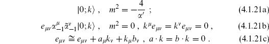
Let us see how this works for the first two levels of the open string in flat spacetime, not necessarily assuming D = 26. The only relevant terms are

At the lowest mass level, the only state is |0;k . The only nontrivial condition at this level is = 0, giving m² = A/′. There are no null states at this level — the Virasoro generators in the spurious state (4.1.8) all contain raising operators. Thus there is one equivalence class, corresponding to a scalar particle.

At the next level there are D states

The norm is

We have used

as follows from the Hermiticity of X, and also

as follows from momentum conservation. The timelike excitation has a negative norm.

The condition gives

The other nontrivial physical state condition is

and so k · e = 0. There is a spurious state at this level:

That is, is spurious. There are now three cases:

  (i)  If A > –1, the mass-squared is positive. Going to the rest frame, the physical state condition removes the negative norm timelike polarization. The spurious state (4.1.18) is not physical, k · k 0, so there are no null states and the spectrum consists of the D − 1 positive-norm states of a massive vector particle.

 (ii)  If A = −1, the mass-squared is zero. Now k · k = 0 so the spurious state is physical and null. Thus,

This describes the D − 2 positive-norm states of a massless vector particle.

(iii)  If A < −1, the mass-squared is negative. The momentum is spacelike, so the physical state condition removes a positive-norm spacelike polarization. The spurious state is not physical, so we are left with a tachyonic vector particle with D − 2 positive-norm states and one negative-norm state.

Case (iii) is unacceptable. Case (ii) is the same as the light-cone quantization. Case (i) is not the same as the light-cone spectrum, having different masses and an extra state at the first level, but does not have any obvious inconsistency. The difficulty is that there is no known way to give such a theory consistent interactions. Case (ii) is the one of interest in string theory, and the one we will recover from the more general approach of the next section.

The result at the next level is quite interesting: it depends on the constant A and also on the spacetime dimension D. Restricting to the value A = −1 found at the first excited level, the spectrum only agrees with the light-cone spectrum if in addition D = 26. If D > 26, there are negative-norm states; if D < 26 the OCQ spectrum has positive norm but more states than in light-cone quantization. The derivation is left to the reader. The OCQ at A = −1 and D = 26 is in fact the same as light-cone quantization at all mass levels,

as will be shown in section 4.4. It is only in this case that consistent interactions are known.

The extension to the closed string is straightforward. There are two sets of oscillators and two sets of Virasoro generators, so at each level the spectrum is the product of two copies of the open string spectrum (except for the normalization of p² in ). The first two levels are then

The relevant values are again A = −1, D = 26. As in light-cone quantization, there are (D – 2)² massless states forming a traceless symmetric tensor, an antisymmetric tensor, and a scalar.

Mnemonic

For more general string theories, it is useful to have a quick mnemonic for obtaining the zero-point constant. As will be derived in the following sections, the condition can be understood as

That is, one includes the ghost contribution with the ghosts in their ground state |↓, which has = −1. The L₀ generators differ from the Hamiltonian by a shift (2.6.10) proportional to the central charge, but the total central charge is zero in string theory so we can just as well write this condition as

Now apply the mnemonic for zero-point energies given at the end of chapter 2. In particular, the ghosts always cancel the = 0, 1 oscillators because they have the same periodicities but opposite statistics. So the rule is that A is given as the sum of the zero-point energies of the transverse oscillators. This is the same rule as in the light-cone, giving here .

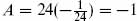Incidentally, for the purposes of counting the physical states (but not for their precise form) one can simply ignore the ghost and = 0, 1 oscillators and count transverse excitations as in the light-cone.

The condition (4.1.22) requires the weight of the matter state to be 1. Since the physical state condition requires the matter state to be a highest weight state, the vertex operator must then be a weight 1 or (1,1) tensor. This agrees with the condition from section 3.6 that the integrated vertex operator be conformally invariant, which gives another understanding of the condition A = −1.

4.2    BRST quantization

We now return to a more systematic study of the spectrum. The condition (4.1.2) is not sufficient to guarantee gauge invariance. It implies invariance for arbitrary fixed choices of g_ab, but this is not the most general gauge. In light-cone gauge, for example, we placed some conditions on X and some conditions on g_ab. To consider the most general possible variation of the gauge condition, we must allow g_ab to be an operator, that is, to depend on the fields in the path integral.

In order to derive the full invariance condition, it is useful to take a more general and abstract point of view. Consider a path integral with a local symmetry. The path integral fields are denoted _i, which in the present case would be X() and g_ab(). Here we use a very condensed notation, where i labels the field and also represents the coordinate . The gauge invariance is , where again includes the coordinate. By assumption the gauge parameters are real, since we can always separate a complex parameter into its real and imaginary parts. The gauge transformations satisfy an algebra

Now fix the gauge by conditions

where once again A includes the coordinate. Following the same Faddeev–Popov procedure as in section 3.3, the path integral becomes

where S₁ is the original gauge-invariant action, S₂ is the gauge-fixing action

and S₃ is the Faddeev–Popov action

We have introduced the field B_A to produce an integral representation of the gauge-fixing (F^A).

There are two things to notice about this action. The first is that it is invariant under the Becchi–Rouet–Stora–Tyutin (BRST) transformation

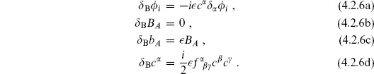
This transformation mixes commuting and anticommuting objects, so that must be taken to be anticommuting. There is a conserved ghost number, which is + 1 for c, −1 for b_A and , and 0 for all other fields. The original action S₁ is invariant by itself, because the action of _B on _i is just a gauge transformation with parameter . The variation of S₂ cancels the variation of b_A in S₃, while the variations of and c in S₃ cancel.

The second key property is that

Now consider a small change F in the gauge-fixing condition. The change in the gauge-fixing and ghost actions gives

where we have written the BRST variation as an anticommutator with the corresponding conserved charge Q_B.

Therefore, physical states must satisfy

In order for this to hold for arbitrary F, it must be that

This is the essential condition: physical states must be BRST-invariant. We have assumed that = Q_B. There are several ways to see that this must indeed be the case. One is that if were different, it would have to be some other symmetry, and there is no candidate. A better argument is that the fields c and b_A are like anticommuting versions of the gauge parameter and Lagrange multiplier B_A, and so inherit their reality properties.

As an aside, we may also add to the action a term proportional to

for any constant matrix M^AB. By the above argument, amplitudes between physical states are unaffected. The integral over B_A now produces a Gaussian rather than a delta function: these are the Gaussian-averaged gauges, which include for example the covariant -gauges of gauge theory.

There is one more key idea. In order to move around in the space of gauge choices, the BRST charge must remain conserved. Thus it must commute with the change in the Hamiltonian,

In order for this to vanish for general changes of gauge, we need

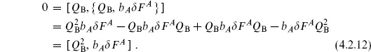
That is, the BRST charge is nilpotent; the possibility = constant is excluded because has ghost number 2. The reader can check that acting twice with the BRST transformation (4.2.6) leaves all fields invariant. In particular,

The product of ghosts is antisymmetric on the indices , and the product of structure functions then vanishes by the Jacobi identity.

We should mention that we have made two simplifying assumptions about the gauge algebra (4.2.1). The first is that the structure constants are constants, independent of the fields, and the second is that the algebra does not have, on the right-hand side, additional terms proportional to the equations of motion. More generally, both of these assumptions break down. In these cases, the BRST formalism as we have described it does not give a nilpotent transformation, and a generalization, the Batalin–Vilkovisky (BV) formalism, is needed. The BV formalism has had various applications in string theory, but we will not have a need for it.

The nilpotence of Q_B has an important consequence. A state of the form

will be annihilated by Q_B for any and so is physical. However, it is orthogonal to all physical states including itself:

if = 0. All physical amplitudes involving such a null state thus vanish. Two physical states that differ by a null state,

will have the same inner products with all physical states and are therefore physically equivalent. So, just as for the OCQ, we identify the true physical space with a set of equivalence classes, states differing by a null state being equivalent. This is a natural construction for a nilpotent operator, and is known as the cohomology of Q_B. Other examples of nilpotent operators are the exterior derivative in differential geometry and the boundary operator in topology. In cohomology, the term closed is often used for states annihilated by Q_B and the term exact for states of the form (4.2.15). Thus, our prescription is

We will see explicitly in the remainder of the chapter that this space has the expected form in string theory. Essentially, the invariance condition removes one set of unphysical X oscillators and one set of ghost oscillators, and the equivalence relation removes the other set of unphysical X oscillators and the other set of ghost oscillators.

Point-particle example

Let us consider an example, the point particle. Expanding out the condensed notation above, the local symmetry is coordinate reparameterization (), so the index just becomes and a basis of infinitesimal transformations is . These act on the fields as

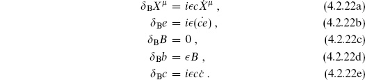
Acting with a second transformation and forming the commutator, we have

From the commutator we have determined the structure function

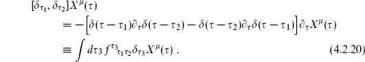
The BRST transformation is then

The gauge e() = 1 is analogous to the unit gauge for the string, using the single coordinate freedom to fix the single component of the tetrad, so F() = 1 −e(). The gauge-fixed action is then

We will find it convenient to integrate B out, thus fixing e = 1. This leaves only the fields X, b, and c, with action

and BRST transformation

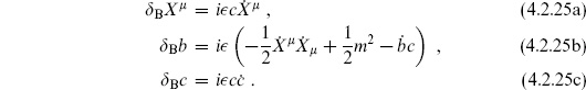
Since B is no longer present, we have used the equation of motion from e to replace B in the transformation law for b. The reader can check that the new transformation (4.2.25) is a symmetry of the action and is nilpotent. This always works when the fields B^A are integrated out, though b is no longer identically zero but is proportional to the equations of motion. This is perfectly satisfactory: = 0 holds as an operator equation, which is what we need.

The canonical commutators are

with , the i being from the Euclidean signature. The Hamiltonian is 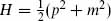, and the Noether procedure gives the BRST operator

The structure here is analogous to what we will find for the string. The constraint (the missing equation of motion) is H = 0, and the BRST operator is c times this.

The ghosts generate a two-state system, so a complete set of states is , where

The action of the BRST operator on these is

From this it follows that the closed states are

and that the exact states are

The closed states that are not exact are

That is, physical states must satisfy the mass-shell condition, but we have two copies of the expected spectrum. In fact, only states |k,↓ satisfying the additional condition

appear in physical amplitudes. The origin of this additional condition is kinematic. For k²+m² 0, the states |k, ↑ are exact — they are orthogonal to all physical states and their amplitudes must vanish identically. So the amplitudes can only be proportional to (k² + m²). But amplitudes in field theory and in string theory, while they may have poles and cuts, never have delta functions (except in D = 2 where the kinematics is special). So they must vanish identically.

4.3    BRST quantization of the string

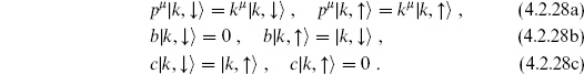
In string theory, the BRST transformation is

The reader can derive this following the point-particle example. To the sum of the Polyakov and ghost actions, add the gauge-fixing term

The transformation _Bb_ab = B_ab becomes (4.3.1) after integrating over B_ab and using the g_ab equation of motion to replace B_ab in the transformation. The Weyl ghost is just a Lagrange multiplier, making b_ab traceless. Again, the reader can check nilpotence up to the equations of motion. The similarity between the string BRST transformation (4.3.1) and the particle case (4.2.25) is evident. Replacing the X with a general matter CFT, the BRST transformation of the matter fields is a conformal transformation with (z) = c(z), while T^m replaces T^X in the transformation of b.

Noether’s theorem gives the BRST current

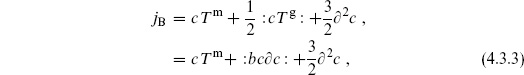
and correspondingly for . The final term in the current is a total derivative and does not contribute to the BRST charge; it has been added by hand to make the BRST current a tensor. The OPEs of the BRST current with the ghost fields and with a general matter tensor field are

The simple poles reflect the BRST transformations (4.3.1) of these fields.

The BRST operator is

By the usual contour argument, the OPE implies

In terms of the ghost modes,

The ordering constant is a^B = a^g = −1, as follows from the anticommutator

There is an anomaly in the gauge symmetry when c^m 26, so we expect some breakdown in the BRST formalism. The BRST current is still conserved: all of the terms in the current (4.3.3) are analytic for any value of the central charge. However, it is no longer nilpotent,

The shortest derivation of this uses the Jacobi identity, exercise 4.3. More directly it follows from the OPE

This requires a bit of calculation, being careful about minus signs from anticommutation. The single pole implies that {Q_B, Q_B} = 0 when c^m = 26. Note also the OPE

which implies that j_B is a tensor only when c^m = 26.

Let us point out some important features. The missing equation of motion is just the vanishing of the generator T_ab of the conformal transformations, the part of the local symmetry group not fixed by the gauge choice. This is a general result. When the gauge conditions fix the symmetry completely, one can show that the missing equations of motion are trivial due to the gauge invariance of the action. When they do not, so that there is a residual symmetry group, the missing equations of motion require its generators to vanish. They must vanish in the sense (4.1.2) of matrix elements, or more generally in the BRST sense. Denote the generators of the residual symmetry group by G_I. The G_I are called constraints; for the string these are L_m and _m. They form an algebra

Associated with each generator is a pair of ghosts, b_I and c^I, where

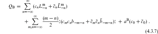
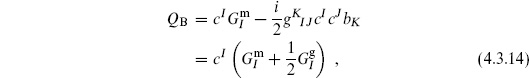
The general form of the BRST operator, as illustrated by the string case (4.3.7), is

where is the matter part of G_I and

is the ghost part. The and satisfy the same algebra (4.3.12) as the G_I. Using the commutators (4.3.12) and (4.3.13), one finds

The last equality follows from the GGG Jacobi identity, which requires g^KIJg^MKL to vanish when antisymmetrized on IJL. We have neglected central charge terms; these need to be checked by hand.

To reiterate, a constraint algebra is a world-sheet symmetry algebra that is required to vanish in physical matrix elements. When we go on to generalize the bosonic string theory in volume two, it will be easiest to do so directly in terms of the constraint algebra, and we will write the BRST charge directly in the form (4.3.14).

BRST cohomology of the string

Let us now look at the BRST cohomology at the lowest levels of the string. The inner product is defined by specifying

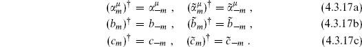
In particular, the Hermiticity of the BRST charge requires that the ghost fields be Hermitean as well. The Hermiticity of the ghost zero modes forces the inner products of the ground state to take the form

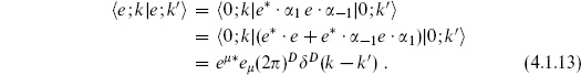
Here |0;k denotes the matter ground state times the ghost ground state |↓, with momentum k. The c₀ and ₀ insertions are necessary for a nonzero result. For example, = 0; the last equality follows because b₀ annihilates both the bra and the ket. The factor of i is needed in the ghost zero-mode inner product for Hermiticity. Inner products of general states are then obtained, as in the earlier calculation (4.1.13), by use of the commutation relations and the adjoints (4.3.17).

We will focus on the open string; the closed string discussion is entirely parallel but requires twice as much writing. As in the point-particle case (4.2.33), we will assert (and later show) that physical states must satisfy the additional condition

This also implies

since Q_B and b₀ both annihilate . The operator L₀ is

where

Thus the L₀ condition (4.3.20) determines the mass of the string. BRST invariance, with the extra condition (4.3.19), implies that every string state is on the mass shell. We will denote by the space of states satisfying the conditions (4.3.19) and (4.3.20). From the commutators {Q_B, b₀} = L₀ and [Q_B, L₀] = 0, it follows that Q_B takes into itself.

The inner product (4.3.18a) is not quite the correct one to use in . It is not well defined: the ghost zero modes give zero, while the ²⁶(k − k′) contains a factor (0) because the momentum support is restricted to the mass shell. Therefore we use in a reduced inner product || in which we simply ignore the X⁰ and ghost zero modes. It is this inner product that will be relevant for the probabilistic interpretation. One can check that Q_B is still Hermitean with the reduced inner product, in the space . Note that the mass-shell condition determines k⁰ in terms of the spatial momentum k (we focus on the incoming case, k⁰ > 0), and that we have used covariant normalization for states.

Let us now work out the first levels of the D = 26 flat spacetime string. At the lowest level, N = 0, we have

This state is invariant,

because every term in Q_B contains either lowering operators or L₀. This also shows that there are no exact states at this level, so each invariant state corresponds to a cohomology class. These are just the states of the tachyon. The mass-shell condition is the same as found in the light-cone quantization of section 1.3 and from the open string vertex operators in section 3.6. The tachyon mass-squared, determined in a heuristic way in chapter 1, is here fixed by the normal ordering constant in Q_B, which is determined by the requirement of nilpotence.

At the next level, N = 1, there are 26 + 2 states,

depending on a 26-vector e and two constants, and . The norm of this state is

Going to an orthogonal basis, there are 26 positive-norm states and 2 negative-norm states. The BRST condition is

The terms proportional to c₀ sum to zero by the mass-shell condition, and are omitted. An invariant state therefore satisfies k · e = = 0. There are 26 linearly independent states remaining, of which 24 have positive norm and 2 have zero norm, being orthogonal to all physical states including themselves. The zero-norm invariant states are created by c₋₁ and k · ₋₁. A general | is of the same form (4.3.25) with constants , so the general BRST-exact state at this level is

Thus the ghost state c₋₁|0;k is BRST-exact, while the polarization is transverse with the equivalence relation 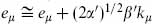. This leaves the 24 positive-norm states expected for a massless vector particle, in agreement with the light-cone quantization and with the OCQ at A = –1.

This pattern is general: there are two extra positive-norm and two extra negative-norm families of oscillators, as compared to the light-cone quantization. The physical state condition eliminates two of these and leaves two combinations with vanishing inner products. These null oscillators are BRST-exact and are removed by the equivalence relation.

An aside: the states b₋₁|0;k and c₋₁|0;k can be identified with the two Faddeev–Popov ghosts that appear in the BRST-invariant quantization of a massless vector field in field theory. The world-sheet BRST operator acts on these states in the same way as the corresponding spacetime BRST operator in gauge field theory. Acting on the full string Hilbert space, the open string BRST operator is then some infinite-dimensional generalization of the spacetime gauge theory BRST invariance, while the closed string BRST operator is a generalization of the spacetime general coordinate BRST invariance, in the free limit.

The generalization to the closed string is straightforward. We restrict attention to the space of states satisfying ¹

implying also

In the closed string,

where

Repeating the earlier exercise, we find at m² = −4/′ the tachyon, and at m² = 0 the 24 × 24 states of the graviton, dilaton, and antisymmetric tensor.

4.4    The no-ghost theorem

In this section we prove that the BRST cohomology of the string has a positive inner product and is isomorphic to the light-cone and OCQ spectra. We are identifying the BRST cohomology as the physical Hilbert space. We will also need to verify, in our study of string amplitudes, that the amplitudes are well defined on the cohomology (that is, that equivalent states have equal amplitudes) and that the S-matrix is unitary within the space of physical states.

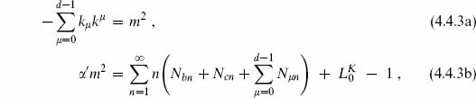
We will work in the general framework described at the end of chapter 3. That is, the world-sheet theory consists of d free X fields including = 0, plus some compact unitary CFT K of central charge 26 − d, plus the ghosts. The Virasoro generators are a sum

By compact we mean that has a discrete spectrum. For example, in the case that K corresponds to strings on a compact manifold, the term ′ p² in L₀ is replaced by the Laplacian − ′∇², which has a discrete spectrum on a compact space.

The general state is labeled

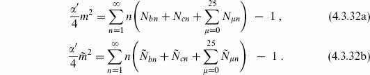
in the open and closed strings respectively, where N (and ) refer to both the d-dimensional and ghost oscillators, k is the d-momentum, and I labels the states of the compact CFT with given boundary conditions. The b₀ condition (4.3.19) or (4.3.29) is imposed as above, implying the mass-shell condition

for the open string and

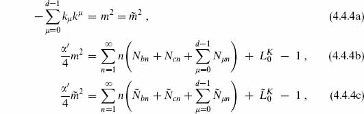
for the closed string. That is, the contributions of the d ≤ ≤ 25 oscillators are replaced by the eigenvalue of or from the compact CFT. The only information we use about the compact CFT is that it is conformally invariant with the appropriate central charge, so there is a nilpotent BRST operator, and that it has a positive inner product. The basis I can be taken to be orthonormal, so the reduced inner products are

Now let us see what we expect for the physical Hilbert space. Define the transverse Hilbert space to consist of those states in that have no longitudinal (X⁰, X¹, b, or c) excitations. Since these oscillators are the source of the indefinite inner product, has a positive inner product. Light-cone gauge-fixing eliminates the longitudinal oscillators directly — the light-cone Hilbert space is isomorphic to , as one sees explicitly in the flat-spacetime case from chapter 1. We will show, in the general case, that the BRST cohomology is isomorphic to . That is, it has the same number of states at each mass level, and has a positive inner product. This is the no-ghost theorem.

Proof

The proof has two parts. The first is to find the cohomology of a simplified BRST operator Q₁, which is quadratic in the oscillators, and the second is to show that the cohomology of the full Q_B is identical to that of Q₁. Define the light-cone oscillators

which satisfy

We will use extensively the quantum number

The number N^lc counts the number of — excitations minus the number of + excitations; it is not a Lorentz generator because the center-of-mass piece has been omitted. We choose a Lorentz frame in which the momentum component k⁺ is nonzero.

Now decompose the BRST generator using the quantum number N^lc:

where Q_j changes N^lc by j units,

Also, each of the Q_j increases the ghost number N^g by one unit:

Expanding out = 0 gives

Each group in parentheses has a different N^lc and so must vanish separately. In particular, Q₁ itself is nilpotent, and so has a cohomology.

Explicitly,

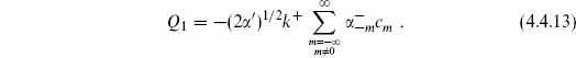
For m < 0 this destroys a + mode and creates a c, and for m > 0 it creates a — mode and destroys a b. One can find the cohomology directly by considering the action of Q₁ in the occupation basis. We will leave this as an exercise, and instead use a standard strategy which will also be useful in generalizing to Q_B. Define

and

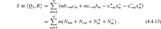
The normal ordering constant is determined by noting that Q₁ and R both annihilate the ground state. Note that Q₁ commutes with S. We can then calculate the cohomology within each eigenspace of S, and the full cohomology is the union of the results. If | is Q₁-invariant with , then for nonzero s

and so | is actually Q₁-exact. Therefore the Q₁ cohomology can be nonzero only at s = 0. By the definition (4.4.15) of S, the s = 0 states have no longitudinal excitations — the s = 0 space is just . The operator Q₁ annihilates all states in , so they are all Q₁-closed and there are no Q₁-exact states in this space. Therefore the cohomology is itself. We have proven the no-ghost theorem, but for the operator Q₁, not Q_B.

The proof had two steps, the first being to show that the cohomology could only come from s = 0 states (the kernel of S), and the second to show that s = 0 states were Q₁-invariant. It is useful to prove the second step in a more abstract way, using the property that all s = 0 states have the same ghost number, in this case −. Suppose S| = 0. Since S and Q₁ commute we have

The state | has ghost number −, so Q₁| has ghost number +. Since S is invertible at this ghost number, it must be that Q₁| = 0 as we wished to show.

It remains to show that the cohomology of Q_B is the same as the cohomology of Q₁. The idea here is to use in place of S the operator

Now, U = {Q₀+Q₋₁, R} lowers N^lc by one or two units. In terms of N^lcy, S is diagonal and U is lower triangular. By general properties of lower triangular matrices, the kernel of S + U can be no larger than the kernel of its diagonal part S. In fact they are isomorphic: if |₀ is annihilated by S, then

is annihilated by S + U. The factors of S⁻¹ make sense because they always act on states of N^lc < 0, where S is invertible. For the same reason, S + U is invertible except at ghost number −. Eqs. (4.4.16) and (4.4.17) can now be applied to Q_B, with S + U replacing S. They imply that the Q_B cohomology is isomorphic to the kernel of S + U, which is isomorphic to the kernel of S, which is isomorphic to the cohomology of Q₁, as we wished to show.

We must still check that the inner product is positive. All terms after the first on the right-hand side of eq. (4.4.19) have strictly negative N^lc. By the commutation relations, the inner product is nonzero only between states whose N^lc adds to zero. Then for two states (4.4.19) in the kernel of S + U,

The positivity of the inner product on the kernel of S + U then follows from that for the kernel of S, and we are done.

After adding the tilded operators to Q_B, N^lc, R, etc., the closed string proof is identical.

BRST–OCQ equivalence

We now prove the equivalence

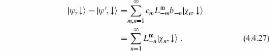
To a state | in the matter Hilbert space, associated the state

from the full matter plus ghost theory. Again the ghost vacuum |↓ is annihilated by all of the ghost lowering operators, b_n for n ≥ 0 and c_n for n > 0. Acting with Q_B,

All terms in Q_B that contain ghost lowering operators drop out, and the constant in the n = 0 term is known from the mode expansion of Q_B, eq. (4.3.7). Each OCQ physical state thus maps to a BRST-closed state. The ordering constant A = −1 arises here from the L₀ eigenvalue of the ghost vacuum.

To establish the equivalence (4.4.21), we need to show more. First, we need to show that we have a well-defined map of equivalence classes: that if and ′ are equivalent OCQ physical states, they map into the same BRST class:

must be BRST-exact. By (4.4.23), this state is BRST-closed. Further, since |′ – | is OCQ null, the state (4.4.24) has zero norm. From the BRST no-ghost theorem, the inner product on the cohomology is positive, so a zero-norm closed state is BRST-exact, as we needed to show.

To conclude that we have an isomorphism, we need to show that the map is one-to-one and onto. One-to-one means that OCQ physical states and ′ that map into the same BRST class must be in the same OCQ class — if

then | – |′ must be OCQ null. To see this, expand

| has ghost number −, so the ellipsis stands for terms with at least one c and two b excitations. Insert this into the form (4.4.25) and keep on both sides only terms with the ghost ground state. This gives

Terms with ghost excitations must vanish separately, and so have been omitted. Thus, is OCQ null, and the map is one-to-one.

Finally, we must show that the map is onto, that every Q_B class contains at least one state of the form (4.4.22). In fact, the specific representatives (4.4.19), the states annihilated by S + U, are of this form. To see this, consider the quantum number N′ = 2N⁻ + N_b + N_c, involving the total numbers of −, b, and c excitations. The operator R has N′ = −1: terms in R with m > 0 reduce N_c by one unit and terms with m < 0 reduce N⁻ by one unit and increase N_b by one unit. Examining Q₀ + Q₋₁, one finds various terms with N′ = 1, but no greater. So U = {R, Q₀ + Q₋₁} cannot increase N′. Examining the state (4.4.19), and noting that S and |₀ have N′ = 0, we see that all terms on the right-hand side have N′ ≤ 0. By definition N′ is nonnegative, so it must be that N′| = 0. This implies no −, b, or c excitations, and so this state is of the form (4.4.22). Thus the equivalence (4.4.21) is shown.

The full power of the BRST method is needed for understanding the general structure of string amplitudes. However, for many practical purposes it is a great simplification to work with the special states of the form |, ↓, and so it is useful to know that every BRST class contains at least one state in which the ghost modes are unexcited. We will call these OCQ-type states.

The OCQ physical state condition (4.1.5) requires that the matter state be a highest weight state with L₀ = 1. The corresponding vertex operator is a weight-1 tensor field ^m constructed from the matter fields. Including the ghost state |↓, the full vertex operator is c^m. For the closed string the full vertex operator is c^m with ^m a (1, 1) tensor. The matter part of the vertex operator is the same as found in the Polyakov formalism in section 3.6, while the ghost part has a simple interpretation that we will encounter in the next chapter.

Eq. (4.4.19) defines an OCQ-physical state in each cohomology class. For the special case of flat spacetime this state can be constructed more explicitly by using the Del Giudice–Di Vecchia–Fubini (DDF) operators. To explain these we will need to develop some more vertex operator technology, so this is deferred to chapter 8.

Exercises

4.1 Extend the OCQ, for A = −1 and general D, to the second excited level of the open string. Verify the assertions made in the text about extra positive- and negative-norm states.

4.2 (a) In the OCQ, show that the state is physical (and therefore null) if | is a highest weight state with = 0.
(b) Show that the state 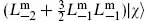is physical and null if | is a highest weight state with = −1.

4.3 By writing out terms, demonstrate the Jacobi identity

This is the sum of cyclic permutations, with commutators or anticommutators as appropriate, and minus signs from anticommutation. Use the Jacobi identity and the (anti)commutators (2.6.24) and (4.3.6) of b_n with L_n and Q_B to show that {[Q_B, L_m], b_n} vanishes when the total central charge is zero. This implies that [Q_B, L_m] contains no c modes. However, this commutator has N^g = 1, and so it must vanish: the charge Q_B is conformally invariant. Now use the Q_BQ_Bb_n Jacobi identity in the same way to show that Q_B is nilpotent when the total central charge is zero.

4.4 In more general situations, one encounters graded Lie algebras, with bosonic generators (fermion number F_I even) and fermionic generators (F_I odd). The algebra of constraints is

Construct a nilpotent BRST operator. You will need bosonic ghosts for the fermionic constraints.

4.5 (a) Carry out the BRST quantization for the first two levels of the closed string explicitly.
(b) Carry out the BRST quantization for the third level of the open string, m² = 1/′.

4.6 (a) Consider the operator , obtained by truncating Q₁ to the m = ±1 oscillators only. Calculate the cohomology of Q′ directly, by considering its action on a general linear combination of the states

(b) Generalize this to the full Q₁.

__________

¹  S. Weinberg has pointed out that the simple argument given at the end of section 4.2 would only lead to the weaker condition = 0. Nevertheless, we shall see from the detailed form of string amplitudes in chapter 9 that there is a projection onto states satisfying conditions (4.3.29).