2
Computing Software Basics

---

This chapter discusses some computing basics starting with computing languages, number representations, and programming tools. The limits and consequences of using floating-point numbers are explored. Related topics dealing with hardware basics are found in Chapter 10.

---

2.1 Making Computers Obey

The best programs are written so that computing machines can perform them quickly and human beings can understand them clearly. A programmer is ideally an essayist who works with traditional aesthetic and literary forms as well as mathematical concepts, to communicate the way that an algorithm works and to convince a reader that the results will be correct.

Donald E. Knuth

As anthropomorphic as your view of your computer may be, keep in mind that computers always do exactly as they are told. This means that you must tell them exactly everything they have to do. Of course, the programs you run may have such convoluted logic that you may not have the endurance to figure out the details of what you have told the computer to do, but it is always possible in principle. So your first problem is to obtain enough understanding so that you feel well enough in control, no matter how illusionary, to figure out what the computer is doing.

Before you tell the computer to obey your orders, you need to understand that life is not simple for computers. The instructions they understand are in a basic machine language¹⁾ that tells the hardware to do things like move a number stored in one memory location to another location or to do some simple binary arithmetic. Very few computational scientists talk to computers in a language computers can understand. When writing and running programs, we usually communicate to the computer through shells, in high-level languages (Python, Java, Fortran, C), or through problem-solving environments (Maple, Mathematica, and Matlab). Eventually, these commands or programs are translated into the basic machine language that the hardware understands.

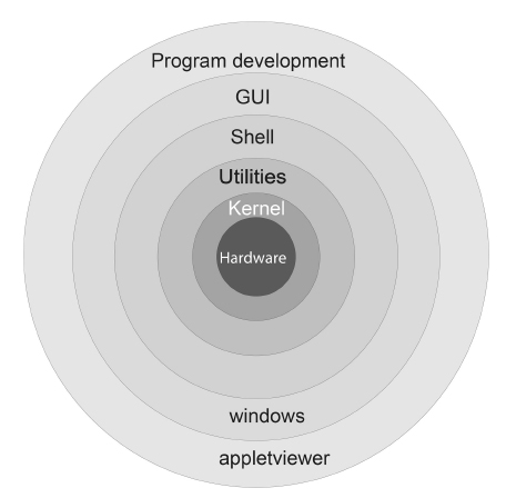
Figure 2.1 A schematic view of a computer’s kernel and shells. The hardware is in the center surrounded by increasing higher level software.

A shell is a command-line interpreter, that is, a set of small programs run by a computer that respond to the commands (the names of the programs) that you key in. Usually you open a special window to access the shell, and this window is called a shell as well. It is helpful to think of these shells as the outer layers of the computer's operating system (OS) (Figure 2.1), within which lies a kernel of elementary operations. (The user seldom interacts directly with the kernel, except possibly when installing programs or when building an OS from scratch.) It is the job of the shell to run programs, compilers, and utilities that do things like copying files. There can be different types of shells on a single computer or multiple copies of the same shell running at the same time.

Operating systems have names such as Unix, Linux, DOS, MacOS, and MS Windows. The operating system is a group of programs used by the computer to communicate with users and devices, to store and read data, and to execute programs. The OS tells the computer what to do in an elementary way. The OS views you, other devices, and programs as input data for it to process; in many ways, it is the indispensable office manager. While all this may seem complicated, the purpose of the OS is to let the computer do the nitty-gritty work so that you can think higher level thoughts and communicate with the computer in something closer to your normal everyday language.

When you submit a program to your computer in a high-level language the computer uses a compiler to process it. The compiler is another program that treats your program as a foreign language and uses a built-in dictionary and set of rules to translate it into basic machine language. As you can probably imagine, the final set of instructions is quite detailed and long and the compiler may make several passes through your program to decipher your logic and translate it into a fast code. The translated statements form an object or compiled code, and when linked together with other needed subprograms, form a load module. A load module is a complete set of machine language instructions that can be loaded into the computer’s memory and read, understood, and followed by the computer.

Languages such as Fortran and C use compilers to read your entire program and then translate it into basic machine instructions. Languages such as BASIC and Maple translate each line of your program as it is entered. Compiled languages usually lead to more efficient programs and permit the use of vast subprogram libraries. Interpreted languages give a more immediate response to the user and thereby appear “friendlier.” The Python and Java languages are a mix of the two. When you first compile your program, Python interprets it into an intermediate, universal byte code which gets stored as a PYC (or PYO) file. This file can be transported to and used on other computers, although not with different versions of Python. Then, when you run your program, Python recompiles the byte code into a machine-specific compiled code, which is faster than interpreting your source code line by line.

2.2 Programming Warmup

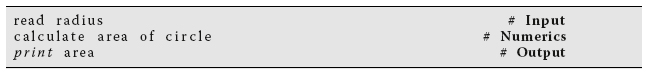
Before we go on to serious work, we want to establish that your local computer is working right for you. Assume that calculators have not yet been invented and that you need a program to calculate the area of a circle. Rather than use any specific language, write that program in pseudocode that can be converted to your favorite language later. The first program tells the computer²⁾:

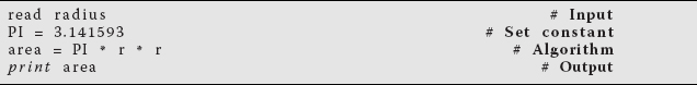
This program cannot really work because it does not tell the computer which circle to consider and what to do with the area. A better program would be

The instruction calculate area of circle has no meaning in most computer languages, so we need to specify an algorithm, that is, a set of rules for the computer to follow:

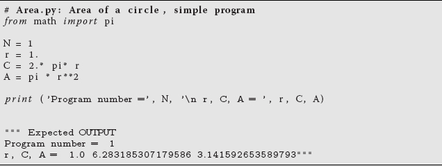
This is a better program, and so let us see how to implement it in Python (other language versions are available online). In Listing 2.1, we give a Python version of our Area program. This is a simple program that outputs to the screen, with its input built into the program.

Listing 2.1 Area.py outputs to the screen, with its input built into the program.

2.2.1 Structured and Reproducible Program Design

Programming is a written art that blends elements of science, mathematics, and computer science into a set of instructions that permit a computer to accomplish a desired task. And now, as published scientific results increasingly rely on computation as an essential element, it is increasingly important that the source of your program itself be available to others so that they can reproduce and extend your results. Reproducibility may not be as exciting as a new discovery, but it is an essential ingredient in science (Hinsen, 2013). In addition to the grammar of a computer language, a scientific program should include a number of essential elements to ensure the program's validity and useability. As with other arts, we suggest that until you know better, you follow some simple rules. A good program should

• Give the correct answers.
• Be clear and easy to read, with the action of each part easy to analyze.
• Document itself for the sake of readers and the programmer.
• Be easy to use.
• Be built up out of small programs that can be independently verified.
• Be easy to modify and robust enough to keep giving correct answers after modification and simple debugging.
• Document the data formats used.
• Use trusted libraries.
• Be published or passed on to others to use and to develop further.

One attraction of object-oriented programming is that it enforces these rules automatically. An elementary way to make any program clearer is to structure it with indentation, skipped lines, and paranetheses placed strategically. This is performed to provide visual clues to the function of the different program parts (the “structures” in structured programming). In fact, Python uses indentations as structure elements as well as for clarity. Although the space limitations of a printed page keep us from inserting as many blank lines as we would prefer, we recommend that you do as we say and not as we do!

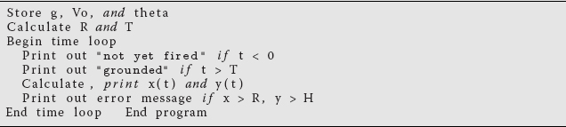
In Figure 2.2, we present basic and detailed flowcharts that illustrate a possible program for computing projectile motion. A flowchart is not meant to be a detailed description of a program but instead a graphical aid to help visualize its logical flow. As such, it is independent of a specific computer language and is useful for developing and understanding the basic structure of a program. We recommend that you draw a flowchart or (second best) write a pseudocode before you write a program. Pseudocode is like a text version of a flowchart that leaves out details and instead focuses on the logic and structures:

2.2.2 Shells, Editors, and Execution

1. To gain some experience with your computer system, use an editor to enter the program Area.py that computes the area of a circle (yes, we know you can copy and paste it, but you may need some exercise before getting to work). Then write your file to a disk by saving it in your home (personal) directory (we advise having a separate subdirectory for each chapter). Note: Readers familiar with Python may want to enter the program AreaFormatted.py instead that uses commands that produce the formatted output.
2. Compile and execute the appropriate version of Area.py.
3. Experiment with your program. For example, see what happens if you leave out decimal points in the assignment statement for r, if you assign r equal to a blank, or if you assign a letter to r. Remember, it is unlikely that you will “break” anything on the computer by making a mistake, and it is good to see how the computer responds when under stress.
4. Change the program so that it computes the volume 4/3 πr³ of a sphere and prints it out with the proper name. Save the modified program to a file it in your personal directory and give it the name Vol.py.
5. Open and execute Vol.py and check that your changes are correct by running a number of trial cases. Good input data are r = 1 and r = 10.
6. Revise Area.py so that it takes input from a file name that you have made up, then writes in a different format to another file you have created, and then reads from the latter file.
7. See what happens when the data type used for output does not match the type of data in the file (e.g., floating point numbers are read in as integers).
8. Revise AreaMod so that it uses a main method (which does the input and output) and a separate function or method for the calculation. Check that you obtain the same answers as before.

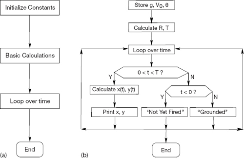
Figure 2.2 A flowchart illustrating a program to compute projectile motion. Plot (a) shows the basic components of the program, and plot (b) shows are some of its details. When writing a program, first map out the basic components, then decide upon the structures, and finally fill in the details. This is called top-down programming.

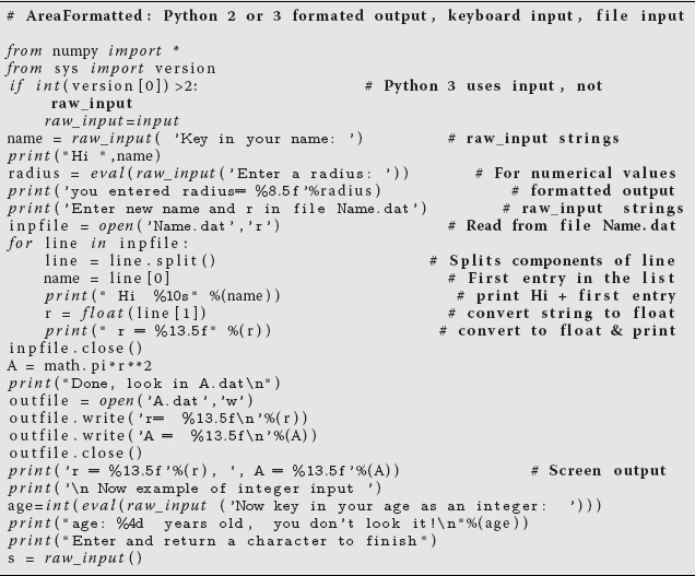
Listing 2.2 AreaFormatted.py does I/O to and from keyboard, as well as from a file. It works with either Python 2 or 3 by switching between raw input and input. Note to read from a file using Canopy, you must right click in the Python run window and choose Change to Editor Directory.

2.3 Python I/O

The simplest I/O with Python is outputting to the screen with the print command (as seen in Area.py, Listing 2.1), and inputting from the keyboard with the input command (as seen in AreaFormatted.py, Listing 2.2). We also see in AreaFormatted.py that we can input strings (literal numbers and letters) by either enclosing the string in quotes (single or double), or by using the raw_input (Python2) or input (Python 3) command without quotes. To print a string with print, place the string in quotes. AreaFormatted.py also shows how to input both a string and numbers from a file. (But be careful if you are using Canopy: you must right click in the Python run window and choose Change to Editor Directory in order to switch the working directory of Canopy's Python shell to your working directory.) The simplest output prints the value of a float just by giving its name:

This uses Python’s default format, which tends to vary depending on the precision of the number being printed. As an alternative, you can control the format of your output. For floats, you need to specify two things. First, how many digits (places) after the decimal point are desired, and second, how many spaces overall should be used for the number:

Here the %6.3f formats a float (which is a double in Python) to be printed in fixed-point notation (the f) with three places after the decimal point and with six places overall (one place for the decimal point, one for the sign, one for the digit before the decimal point, and three for the decimal). The directive %9.6f produces six digits after the decimal place and nine overall.

To print an integer, we need to specify only the total number of digits (there is no decimal part), and we do that with the %d (d for digits) format. The % symbol in these output formats indicates a conversion from the computer’s internal format to that used for output. Notice in Listing 2.2 how we read from the keyboard, as well as from a file, and then output to both the screen and file. Beware that if you do not create the file Name.dat, the program will issue (“throw”) an error message of the sort:

IOError: [Errno 2] No such file or directory: ’Name.dat’

Note that we have also use a \n directive here to indicate a new line. Other directives, some of which are demonstrated in Directives.py in Listing 2.3 (and some of which like backspace may not yet work right) are:

\"  double quote

\a  alert (bell)

\f  form feed

\t  horizontal tab

\0NNN  octal NNN

\b  backspace

\n  new line

\v  vertical tab

\\  backslash

\c  no more output

\r  carriage ret

%%  a single %

Listing 2.3 Directives.py illustrates formatting via directives and escape characters.

2.4 Computer Number Representations (Theory)

Computers may be powerful, but they are finite. A problem in computer design is how to represent an arbitrary number using a finite amount of memory space and then how to deal with the limitations arising from this representation. As a consequence of computer memories being based on the magnetic or electronic realizations of a spin pointing up or down, the most elementary units of computer memory are the two binary integers (bits) 0 and 1. This means that all numbers are stored in memory in the binary form, that is, as long strings of 0s and 1s. Accordingly, N bits can store integers in the range [0, 2^N], yet because the sign of the integer is represented by the first bit (a zero bit for positive numbers), the actual range for N-bit integers decreases to [0, 2^N−1].

Long strings of 0s and 1s are fine for computers but are awkward for humans. For this reason, binary strings are converted to octal, decimal, or hexadecimal numbers before the results are communicated to people. Octal and hexadecimal numbers are nice because the conversion maintains precision, but not all that nice because our decimal rules of arithmetic do not work for octals and hexadecimals. Converting to decimal numbers makes the numbers easier for us to work with, but unless the original number is a power of 2, the conversion decreases precision.

A description of a particular computer’s system or language normally states the word length, that is, the number of bits used to store a number. The length is often expressed in bytes, (a mouthful of bits) where

Memory and storage sizes are measured in bytes, kilobytes, megabytes, gigabytes, terabytes, and petabytes (10¹⁵). Some care should be taken here by those who chose to compute sizes in detail, because K does not always mean 1000:

(2.1)

This is often (and confusingly) compensated for when memory size is stated in K, for example,

Conveniently, 1 byte is also the amount of memory needed to store a single letter like “a,” which adds up to a typical printed page requiring ∼3 kB.

The memory chips in some older personal computers used 8-bit words, with modern PCs using 64 bits. This means that the maximum integer was a rather small 2⁷ = 128 (7 because 1 bits is used for the sign). Using 64 bits permits integers in the range 1−2⁶³ 10¹⁹. While at first this may seem like a large range, it really is not when compared to the range of sizes encountered in the physical world. As a case in point, the size of the universe compared to the size of a proton covers a scale of 10⁴¹. Trying to store a number larger than the hardware or software was designed for (overflow) was common on older machines, but is less so now. An overflow is sometimes accompanied by an informative error message, and sometimes not.

2.4.1 IEEE Floating-Point Numbers

Real numbers are represented on computers in either fixed-point or floating-point notation. Fixed-point notation can be used for numbers with a fixed number of places beyond the decimal point (radix) or for integers. It has the advantages of being able to use two’s complement arithmetic and being able to store integers exactly.³⁾ In the fixed-point representation with N bits and with a two’s complement format, a number is represented as

(2.2)

where n + m = N − 2. That is, 1 bit is used to store the sign, with the remaining (N − 1) bits used to store the α_i values (the powers of 2 are understood). The particular values for N, m, and n are machine dependent. Integers are typically 4 bytes (32 bits) in length and in the range

(2.3)

An advantage of the representation (2.2) is that you can count on all fixed-point numbers having the same absolute error of 2^−m−1 (the term left off the right-hand end of (2.2)). The corresponding disadvantage is that small numbers (those for which the first string of α values are zeros) have large relative errors. Because relative errors in the real world tend to be more important than absolute ones, integers are used mainly for counting purposes and in special applications (like banking).

Most scientific computations use double-precision floating-point numbers with 64 bits = 8 B. The floating-point representation of numbers on computers is a binary version of what is commonly known as scientific or engineering notation. For example, the speed of light c = +2.997 924 58 × 10⁸ m/s in scientific notation and +0.299 792 458 × 10⁹ or 0.299 795 498 E09 m/s in engineering notation. In each of these cases, the number in front is called the mantissa and contains nine significant figures. The power to which 10 is raised is called the exponent, with the plus sign in front a reminder that these numbers may be negative.

Floating-point numbers are stored on the computer as a concatenation (juxtaposition) of a sign bit, an exponent, and a mantissa. Because only a finite number of bits are stored, the set of floating-point numbers that the computer can store exactly, machine numbers (the hash marks in Figure 2.3), does not cover the entire the set of real numbers. In particular, machine numbers have a maximum and a minimum (the shading in Figure 2.3). If you exceed the maximum, an error condition known as overflow occurs; if you fall below the minimum, an error condition known as underflow occurs. In the latter case, the software and hardware may be set up so that underflows are set to zero without your even being told. In contrast, overflows usually halt a program’s execution.

The actual relation between what is stored in memory and the value of a floating-point number is somewhat indirect, with there being a number of special cases and relations used over the years. In fact, in the past each computer OS and each computer language contained its own standards for floating-point numbers. Different standards meant that the same program running correctly on different computers could give different results. Although the results usually were only slightly different, the user could never be sure if the lack of reproducibility of a test case was as a result of the particular computer being used or to an error in the program’s implementation.

Figure 2.3 The limits of single-precision floating-point numbers and the consequences of exceeding these limits (not to scale). The hash marks represent the values of numbers that can be stored; storing a number in between these values leads to truncation error. The shaded areas correspond to over- and underflow.

In 1987, the Institute of Electrical and Electronics Engineers (IEEE) and the American National Standards Institute (ANSI) adopted the IEEE 754 standard for floating-point arithmetic. When the standard is followed, you can expect the primitive data types to have the precision and ranges given in Table 2.1. In addition, when computers and software adhere to this standard, and most do now, you are guaranteed that your program will produce identical results on different computers. Nevertheless, because the IEEE standard may not produce the most efficient code or the highest accuracy for a particular computer, sometimes you may have to invoke compiler options to demand that the IEEE standard be strictly followed for your test cases. After you know that the code is okay, you may want to run with whatever gives the greatest speed and precision.

Table 2.1 The IEEE 754 Standard for Primitive Data Types.

Name	Type	Bits	Bytes	Range
boolean	Logical	1		true or false
char	String	16	2	'\u0000' ↔ '\uFFFF' (ISO Unicode)
byte	Integer	8	1	−128 ↔ +127
short	Integer	16	2	−32 768 ↔ +32 767
int	Integer	32	4	−2 147 483 648 ↔ +2 147 483 647
long	Integer	64	8	−9 223 372 036 854 775 808 ↔ 9 223 372 036 854 775 807
float	Floating	32	4	±1.401 298 × 10−45 ↔ ±3.402 923 × 1038
double	Floating	64	8	±4.940 656 458 412 465 44 × 10−324 ↔ ±1.797 693 134 862 315 7 × 10308

There are actually a number of components in the IEEE standard, and different computer or chip manufacturers may adhere to only some of them. Furthermore, Python as it develops may not follow all standards, but probably will in time. Normally, a floating-point number x is stored as

(2.4)

that is, with separate entities for the sign s, the fractional part of the mantissa f, and the exponential field e. All parts are stored in the binary form and occupy adjacent segments of a single 32-bit word for singles or two adjacent 32-bit words for doubles. The sign s is stored as a single bit, with s = 0 or 1 for a positive or a negative sign. Eight bits are used to stored the exponent e, which means that e can be in the range 0 ≤ e ≤ 255. The endpoints, e = 0 and e = 255, are special cases (Table 2.2). Normal numbers have 0 < e < 255, and with them the convention is to assume that the mantissa’s first bit is a 1, so only the fractional part f after the binary point is stored. The representations for subnormal numbers and for the special cases are given in Table 2.2.

Note that the values ±INF and NaN are not numbers in the mathematical sense, that is, objects that can be manipulated or used in calculations to take limits and such. Rather, they are signals to the computer and to you that something has gone awry and that the calculation should probably stop until you straighten things out. In contrast, the value −0 can be used in a calculation with no harm. Some languages may set unassigned variables to −0 as a hint that they have yet to be assigned, although it is best not to count on that!

Because the uncertainty (error) is only in the mantissa and not in the exponent, the IEEE representations ensure that all normal floating-point numbers have the same relative precision. Because the first bit of a floating point number is assumed to be 1, it does not have to be stored, and computer designers need only recall that there is a phantom bit 1 there to obtain an extra bit of precision. During the processing of numbers in a calculation, the first bit of an intermediate result may become zero, but this is changed before the final number is stored. To repeat, for normal cases, the actual mantissa (1.f in binary notation) contains an implied 1 preceding the binary point.

Table 2.2 Representation scheme for normal and abnormal IEEE singles.

Number name	Values of s, e, and f	Value of single
Normal	0 < e < 255	(−l)s × 2e−127 × 1.f
Subnormal	e = 0, f ≠ 0	(−l)s × 2−126 × 0.f
Signed zero (±0)	e = 0, f = 0	(−l)s × 0.0
+∞	s = 0, e = 255, f = 0	+INF
−∞	s = l, e = 255, f = 0	−INF
Not a number	s = u, e = 255, f ≠ 0	NaN

Finally, in order to guarantee that the stored biased exponent e is always positive, a fixed number called the bias is added to the actual exponent p before it is stored as the biased exponent e. The actual exponent, which may be negative, is

(2.5)

2.4.1.1 Examples of IEEE Representations

There are two basic IEEE floating-point formats: singles and doubles. Singles or floats is shorthand for single-precision floating-point numbers, and doubles is shorthand for double-precision floating-point numbers. (In Python, however, all floats are double precision.) Singles occupy 32 bits overall, with 1 bit for the sign, 8 bits for the exponent, and 23 bits for the fractional mantissa (which gives 24-bit precision when the phantom bit is included). Doubles occupy 64 bits overall, with 1 bit for the sign, 10 bits for the exponent, and 53 bits for the fractional mantissa (for 54-bit precision). This means that the exponents and mantissas for doubles are not simply double those of floats, as we see in Table 2.1. (In addition, the IEEE standard also permits extended precision that goes beyond doubles, but this is all complicated enough without going into that right now.)

To see the scheme in practice, consider the 32-bit representation (2.4):

The sign bit s is in bit position 31, the biased exponent e is in bits 30−23, and the fractional part of the mantissa f is in bits 22−0. Because 8 bits are used to store the exponent e and because 2⁸ = 256, e has the range

(2.6)

The values e = 0 and 255 are special cases. With bias = 127₁₀, the full exponent

(2.7)

and, as indicated in Table 2.1, singles have the range

(2.8)

The mantissa f for singles is stored as the 23 bits in positions 22−0. For normal numbers, that is, numbers with 0 < e < 255, f is the fractional part of the mantissa, and therefore the actual number represented by the 32 bits is

(2.9)

Subnormal numbers have e = 0, f ≠ 0. For these, f is the entire mantissa, so the actual number represented by these 32 bits is

(2.10)

The 23 bits m₂₂ − m₀, which are used to store the mantissa of normal singles, correspond to the representation

(2.11)

with 0.f used for subnormal numbers. The special e = 0 representations used to store ±0 and ±∞ are given in Table 2.2.

To see how this works in practice (Figure 2.3), the largest positive normal floating-point number possible for a 32-bit machine has the maximum value e = 254 (the value 255 being reserved) and the maximum value for f:

(2.12)

where we have grouped the bits for clarity. After putting all the pieces together, we obtain the value shown in Table 2.1:

(2.13)

Likewise, the smallest positive floating-point number possible is subnormal (e = 0) with a single significant bit in the mantissa:

(2.14)

This corresponds to

(2.15)

In summary, single-precision (32-bit or 4-byte) numbers have six or seven decimal places of significance and magnitudes in the range

(2.16)

Doubles are stored as two 32-bit words, for a total of 64 bits (8 B). The sign occupies 1 bit, the exponent e, 11 bits, and the fractional mantissa, 52 bits:

As we see here, the fields are stored contiguously, with part of the mantissa f stored in separate 32-bit words. The order of these words, and whether the second word with f is the most or least significant part of the mantissa, is machine-dependent. For doubles, the bias is quite a bit larger than for singles,

(2.17)

Table 2.3 Representation scheme for IEEE doubles.

Number name	Values of s, e, and f	Value of double
Normal	0 < e < 2047	(−l)s × 2e−1023 × 1.f
Subnormal	e = 0, f ≠ 0	(−l)s × 2−1022 × 0.f
Signed zero	e = 0, f = 0	(−1)s × 0.0
+∞	s = 0, e = 2047, f = 0	+INF
−∞	s = l, e = 2047, f = 0	−INF
Not a number	s = u, e = 2047, f ≠ 0	NaN

so the actual exponent p = e − 1023.

The bit patterns for doubles are given in Table 2.3, with the range and precision given in Table 2.1. To repeat, if you write a program with doubles, then 64 bits (8 bytes) will be used to store your floating-point numbers. Doubles have approximately 16 decimal places of precision (1 part in 2⁵²) and magnitudes in the range

(2.18)

If a single-precision number x is larger than 2¹²⁸, a fault condition known as an overflow occurs (Figure 2.3). If x is smaller than 2⁻¹²⁸, an underflow occurs. For overflows, the resulting number x_c may end up being a machine-dependent pattern, not a number (NAN), or unpredictable. For underflows, the resulting number x_c is usually set to zero, although this can usually be changed via a compiler option. (Having the computer automatically convert underflows to zero is usually a good path to follow; converting overflows to zero may be the path to disaster.) Because the only difference between the representations of positive and negative numbers on the computer is the sign bit of 1 for negative numbers, the same considerations hold for negative numbers.

In our experience, serious scientific calculations almost always require at least 64-bit (double-precision) floats. And if you need double precision in one part of your calculation, you probably need it all over, which means double-precision library routines for methods and functions.

2.4.2 Python and the IEEE 754 Standard

Python is a relatively recent language with changes and extensions occurring as its use spreads and as its features mature. It should be no surprise then that Python does not at present adhere to all aspects, and especially the special cases, of the IEEE 754 standard. Probably the most relevant difference for us is that Python does not support single (32 bits) precision floating-point numbers. So when we deal with a data type called a float in Python, it is the equivalent of a double in the IEEE standard. Because singles are inadequate for most scientific computing, this is not a loss. However be wary, if you switch over to Java or C you should declare your variables as doubles and not as floats. While Python eliminates single-precision floats, it adds a new data type complex for dealing with complex numbers. Complex numbers are stored as pairs of doubles and are quite useful in science.

The details of how closely Python adheres to the IEEE 754 standard depend upon the details of Python's use of the C or Java language to power the Python interpreter. In particular, with the recent 64 bits architectures for CPUs, the range may even be greater than the IEEE standard, and the abnormal numbers (±INF, NaN) may differ. Likewise, the exact conditions for overflows and underflows may also differ. That being the case, the exploratory exercises to follow become all that more interesting because we cannot say that we know what results you should obtain!

2.4.3 Over and Underflow Exercises

1. Consider the 32-bit single-precision floating-point number A:

   

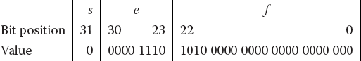
   1. a) What are the (binary) values for the sign s, the exponent e, and the fractional mantissa f? (Hint: e₁₀ = 14.)
   2. b) Determine decimal values for the biased exponent e and the true exponent p.
   3. c) Show that the mantissa of A equals 1.625 000.
   4. d) Determine the full value of A.
2. Write a program that determines the underflow and overflow limits (within a factor of 2) for Python on your computer. Here is a sample pseudocode

   

   
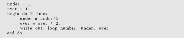
   You may need to increase N if your initial choice does not lead to underflow and overflow. (Notice that if you want to be more precise regarding the limits of your computer, you may want to multiply and divide by a number smaller than 2.)
   1. a) Check where under- and overflow occur for double-precision floating-point numbers (floats). Give your answer in decimal.
   2. b) Check where under- and overflow occur for double-precision floating-point numbers.
   3. c) Check where under- and overflow occur for integers. Note: There is no exponent stored for integers, so the smallest integer corresponds to the most negative one. To determine the largest and smallest integers, you must observe your program’s output as you explicitly pass through the limits. You accomplish this by continually adding and subtracting 1. (Because integer arithmetic uses two's complement arithmetic, you should expect some surprises.)

2.4.4 Machine Precision (Model)

A major concern of computational scientists is that the floating-point representation used to store numbers is of limited precision. As we have shown for a 32-bit-word machine, single-precision numbers are good to 6–7 decimal places, while doubles are good to 15–16 places. To see how limited precision affects calculations, consider the simple computer addition of two single-precision numbers:

(2.19)

The computer fetches these numbers from memory and stores the bit patterns

(2.20)

(2.21)

in working registers (pieces of fast-responding memory). Because the exponents are different, it would be incorrect to add the mantissas, and so the exponent of the smaller number is made larger while progressively decreasing the mantissa by shifting bits to the right (inserting zeros) until both numbers have the same exponent:

(2.22)

(2.23)

Because there is no room left to store the last digits, they are lost, and after all this hard work the addition just gives 7 as the answer (truncation error in Figure 2.3). In other words, because a 32-bit computer stores only 6 or 7 decimal places, it effectively ignores any changes beyond the sixth decimal place.

The preceding loss of precision is categorized by defining the machine precision _m as the maximum positive number that, on the computer, can be added to the number stored as 1 without changing that stored 1:

(2.24)

where the subscript c is a reminder that this is a computer representation of 1. Consequently, an arbitrary number x can be thought of as related to its floating-point representation x_c by

(2.25)

where the actual value for is not known. In other words, except for powers of 2 that are represented exactly, we should assume that all single-precision numbers contain an error in the sixth decimal place and that all doubles have an error in the 15th place. And as is always the case with errors, we must assume that we really do not know what the error is, for if we knew, then we would eliminate it! Consequently, the arguments we are about to put forth regarding errors should be considered approximate, but that is to be expected for unknown errors.

2.4.5 Experiment: Your Machine’s Precision

Write a program to determine the machine precision _m of your computer system within a factor of 2. A sample pseudocode is

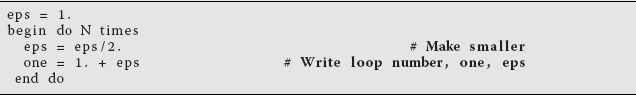
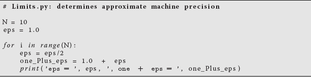
A Python implementation is given in Listing 2.4, while a more precise one is Byte-Limit.py on the instructor’s guide.

Listing 2.4 Limits.py determines machine precision within a factorof 2.

1. Determine experimentally the precision of double-precision floats.
2. Determine experimentally the precision of complex numbers.

To print out a number in the decimal format, the computer must convert from its internal binary representation. This not only takes time, but unless the number is an exact power of 2, leads to a loss of precision. So if you want a truly precise indication of the stored numbers, you should avoid conversion to decimals and instead print them out in octal or hexadecimal format (\0NNN).

2.5 Problem: Summing Series

A classic numerical problem is the summation of a series to evaluate a function. As an example, consider the infinite series for sin x:

(2.26)

Your problem is to use just this series to calculate sin x for x < 2π and x > 2π, with an absolute error in each case of less than 1 part in 10⁸. While an infinite series is exact in a mathematical sense, it is not a good algorithm because errors tend to accumulate and because we must stop summing at some point. An algorithm would be the finite sum

(2.27)

But how do we decide when to stop summing? (Do not even think of saying, “When the answer agrees with a table or with the built-in library function.”) One approach would be to stop summing when the next term is smaller than the precision desired. Clearly then, if x is large, this would require large N as well. In fact, for really large x, one would have to go far out in the series before the terms start decreasing.

2.5.1 Numerical Summation (Method)

Never mind that the algorithm (2.27) indicates that we should calculate and then divide it by This is not a good way to compute. On the one hand, both and can get very large and cause overflows, despite the fact that their quotient may not be large. On the other hand, powers and factorials are very expensive (time-consuming) to evaluate on the computer. Consequently, a better approach is to use a single multiplication to relate the next term in the series to the previous one:

(2.28)

While we want to establish absolute accuracy for sin x, that is not so easy to do. What is easy to do is to assume that the error in the summation is approximately the last term summed (this assumes no round-off error, a subject we talk about in Chapter 3). To obtain a relative error of 1 part in 10⁸, we then stop the calculation when

(2.29)

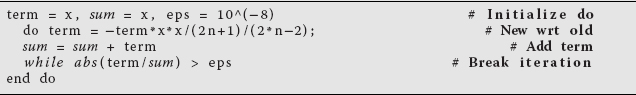
where “term” is the last term kept in the series (2.27) and “sum” is the accumulated sum of all the terms. In general, you are free to pick any tolerance level you desire, although if it is too close to, or smaller than, machine precision, your calculation may not be able to attain it. A pseudocode for performing the summation is

2.5.2 Implementation and Assessment

1. Write a program that implements this pseudocode for the indicated x values. Present the results as a table with headings x imax sum |sum- sin(x)|/sin(x), where sin(x) is the value obtained from the built-in function. The last column here is the relative error in your computation. Modify the code that sums the series in a “good way” (no factorials) to one that calculates the sum in a “bad way” (explicit factorials).
2. Produce a table as above.
3. Start with a tolerance of 10⁻⁸ as in (2.29).
4. Show that for sufficiently small values of x, your algorithm converges (the changes are smaller than your tolerance level) and that it converges to the correct answer.
5. Compare the number of decimal places of precision obtained with that expected from (2.29).
6. Without using the identity , show that there is a range of somewhat large values of x for which the algorithm converges, but that it converges to the wrong answer.
7. Show that as you keep increasing x, you will reach a regime where the algorithm does not even converge.
8. Now make use of the identity to compute sin x for large x values where the series otherwise would diverge.
9. Repeat the calculation using the “bad” version of the algorithm (the one that calculates factorials) and compare the answers.
10. Set your tolerance level to a number smaller than machine precision and see how this affects your conclusions.

1) The Beginner’s All-Purpose Symbolic Instruction Code (BASIC) programming language of the original PCs should not be confused with basic machine language.

2) Comments placed in the field to the right are for your information and not for the computer to act upon.

3) The two’s complement of a binary number is the value obtained by subtracting the number from 2^N for an N-bit representation. Because this system represents negative numbers by the two’s complement of the absolute value of the number, additions and subtractions can be made without the need to work with the sign of the number.