10
High-Performance Hardware and Parallel Computers

---

This chapter discusses a number of topics associated with high-performance computing (HPC) and parallel computing. Although this may sound like something only specialists should be reading, using history as a guide, present HPC hardware and software will be desktop machines in less than a decade, and so you may as well learn these things now. We start with a discussion of a high-performance computer’s memory and central processor design, and then examine various general aspects of parallel computing. Chapter 11 goes on to discuss some practical programming aspects of HPC and parallel computing. HPC is a broad subject, and our presentation is brief and given from a practitioner’s point of view. The text (Quinn, 2004) surveys parallel computing and message passing interface from a computer science point of view. Other references on parallel computing include van de Velde (1994); Fox (1994), and Pancake (1996).

10.1 High-Performance Computers

By definition, supercomputers are the fastest and most powerful computers available, and at present, the term refers to machines with hundreds of thousands of processors. They are the superstars of the high-performance class of computers. Personal computers (PCs) small enough in size and cost to be used by an individual, yet powerful enough for advanced scientific and engineering applications, can also be high-performance computers. We define high-performance computers as machines with a good balance among the following major elements:

• Multistaged (pipelined) functional units,
• Multiple central processing units (CPUs),
• Multiple cores,
• Fast central registers,
• Very large, fast memories,
• Very fast communication among functional units,
• Vector, video, or array processors,
• Software that integrates the above effectively and efficiently.

As the simplest example, it makes little sense to have a CPU of incredibly high speed coupled to a memory system and software that cannot keep up with it.

10.2 Memory Hierarchy

An idealized model of computer architecture is a CPU sequentially executing a stream of instructions and reading from a continuous block of memory. To illustrate, in Figure 10.1 we have a vector A[ ] and an array M[.. , ..] loaded in memory and about to be processed. The real world is more complicated than this. First, arrays are not stored in 2D blocks, but rather in the linear order. For instance, in Python, Java, and C it is in row-major order:

[10.1]

In Fortran, it is in column-major order:

[10.2]

Second, as illustrated in Figures 10.2 and 10.3, the values for the matrix elements may not even be in the same physical place. Some may be in RAM, some on the disk, some in cache, and some in the CPU. To give these words more meaning, in Figures 10.3 and 10.2 we show simple models of the memory architecture of a high-performance computer. This hierarchical arrangement arises from an effort to balance speed and cost, with fast, expensive memory supplemented by slow, less expensive memory. The memory architecture may include the following elements:

CPU Central processing unit, the fastest part of the computer. The CPU consists of a number of very high-speed memory units called registers containing the instructions sent to the hardware to do things like fetch, store, and operate on data. There are usually separate registers for instructions, addresses, and operands (current data). In many cases, the CPU also contains some specialized parts for accelerating the processing of floating-point numbers.

Cache A small, very fast bit of memory that holds instructions, addresses, and data in their passage between the very fast CPU registers and the slower RAM (also called a high-speed buffer). This is seen in the next level down the pyramid in Figure 10.2. The main memory is also called dynamic RAM (DRAM), while the cache is called static RAM (SRAM). If the cache is used properly, it can greatly reduce the time that the CPU waits for data to be fetched from memory.

Cache lines The data transferred to and from the cache or CPU are grouped into cache or data lines. The time it takes to bring data from memory into the cache is called latency.

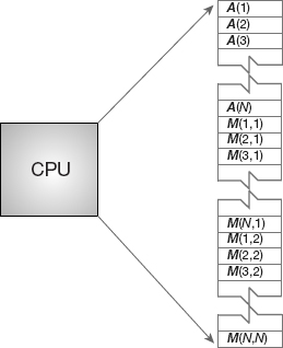
Figure 10.1 The logical arrangement of the CPU and memory showing a Fortran array A(N) and matrix M(N, N) loaded into memory.

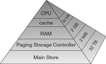
Figure 10.2 Typical memory hierarchy for a single-processor, high-performance computer (B = bytes, k, M, G, T = kilo, mega, giga, tera).

RAM Random-access or central memory is in the middle of the memory hierarchy in Figure 10.2. RAM is fast because its addresses can be accessed directly in random order, and because no mechanical devices are needed to read it.

Pages Central memory is organized into pages, which are blocks of memory of fixed length. The operating system labels and organizes its memory pages much like we do the pages of a book; they are numbered and kept track of with a table of contents. Typical page sizes range from 4 to 16 kB, but on supercomputers they may be in the MB range.

Hard disk Finally, at the bottom of the memory pyramid is permanent storage on magnetic disks or optical devices. Although disks are very slow compared to RAM, they can store vast amounts of data and sometimes compensate for their slower speeds by using a cache of their own, the paging storage controller.

Virtual memory True to its name, this is a part of memory you will not find in our figures because it is virtual. It acts like RAM but resides on the disk.

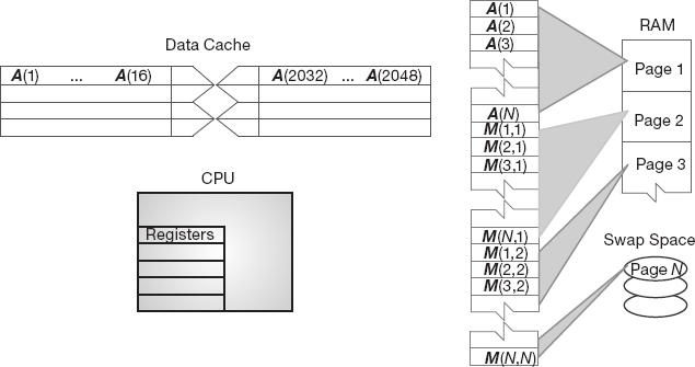
Figure 10.3 The elements of a computer’s memory architecture in the process of handling matrix storage.

When we speak of “fast” and “slow” memory we are using a time scale set by the clock in the CPU. To be specific, if your computer has a clock speed or cycle time of 1 ns, this means that it could perform a billion operations per second, if it could get its hands on the needed data quickly enough (typically, more than 10 cycles are needed to execute a single instruction). While it usually takes 1 cycle to transfer data from the cache to the CPU, the other types of memories are much slower. Consequently, you can speedup your program by having all needed data available for the CPU when it tries to execute your instructions; otherwise the CPU may drop your computation and go on to other chores while your data gets transferred from lower memory (we talk more about this soon in the discussion of pipelining or cache reuse). Compilers try to do this for you, but their success is affected by your programming style.

As shown in Figure 10.3, virtual memory permits your program to use more pages of memory than can physically fit into RAM at one time. A combination of operating system and hardware maps this virtual memory into pages with typical lengths of 4–16 kB. Pages not currently in use are stored in the slower memory on the hard disk and brought into fast memory only when needed. The separate memory location for this switching is known as swap space (Figure 10.4a).

Observe that when an application accesses the memory location for M[i,j], the number of the page of memory holding this address is determined by the computer, and the location of M[i,j] within this page is also determined. A page fault occurs if the needed page resides on disk rather than in RAM. In this case, the entire page must be read into memory while the least recently used page in RAM is swapped onto the disk. Thanks to virtual memory, it is possible to run programs on small computers that otherwise would require larger machines (or extensive reprogramming). The price you pay for virtual memory is an order-of-magnitude slowdown of your program’s speed when virtual memory is actually invoked. But this may be cheap compared to the time you would have to spend to rewrite your program so it fits into RAM, or the money you would have to spend to buy enough RAM for your problem.

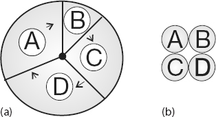
Figure 10.4 (a) Multitasking of four programs in memory at one time. On a SISD computer the programs are executed in round robin order. (b) Four programs in the four separate memories of a MIMD computer.

Virtual memory also allows multitasking, the simultaneous loading into memory of more programs than can physically fit into RAM (Figure 10.4b). Although the ensuing switching among applications uses computing cycles, by avoiding long waits while an application is loaded into memory, multitasking increases total throughout and permits an improved computing environment for users. For example, it is multitasking that permits a windowing system, such as Linux, Apple OS, or Windows, to provide us with multiple windows. Although each window application uses a fair amount of memory, only the single application currently receiving input must actually reside in memory; the rest are paged out to disk. This explains why you may notice a slight delay when switching to an idle window; the pages for the now-active program are being placed into RAM, and the least used application still in memory is simultaneously being paged out.

10.3 The Central Processing Unit

How does the CPU get to be so fast? Often, it utilizes prefetching and pipelining; that is, it has the ability to prepare for the next instruction before the current one has finished. It is like an assembly line or a bucket brigade in which the person filling the buckets at one end of the line does not wait for each bucket to arrive at the other end before filling another bucket. In the same way, a processor fetches, reads, and decodes an instruction while another instruction is executing. Consequently, despite the fact that it may take more than one cycle to perform some operations, it is possible for data to be entering and leaving the CPU on each cycle. To illustrate, Table 10.1 indicates how the operation c = (a + b)/(d × f) is handled. Here the pipelined arithmetic units A1 and A2 are simultaneously doing their jobs of fetching and operating on operands, yet arithmetic unit A3 must wait for the first two units to complete their tasks before it has something to do (during which time the other two sit idle).

Table 10.1 Computation of c = (a + b)/(d × f).

Arithmetic Unit	Step 1	Step 2	Step 3	Step 4
A1	Fetch a	Fetch b	Add	—
A2	Fetch d	Fetch f	Multiply	—
A3	—	—	—	Divide

10.4 CPU Design: Reduced Instruction Set Processors

Reduced instruction set computer (RISC) architecture (also called superscalar) is a design philosophy for CPUs developedfor high-performance computers and now used broadly. It increases the arithmetic speed of the CPU by decreasing the number of instructions the CPU must follow. To understand RISC, we contrast it with CISC (complex instruction set computer) architecture. In the late 1970s, processor designers began to take advantage of very-large-scale integration (VLSI), which allowed the placement of hundreds of thousands of elements on a single CPU chip. Much of the space on these early chips was dedicated to microcode programs written by chip designers and containing machine language instructions that set the operating characteristics of the computer. There were more than 1000 instructions available, and many were similar to higher level programming languages like Pascal and Forth. The price paid for the large number of complex instructions was slow speed, with a typical instruction taking more than 10 clock cycles. Furthermore, a 1975 study by Alexander and Wortman of the XLP compiler of the IBM System/360 showed that about 30 low-level instructions accounted for 99% of the use with only 10 of these instructions accounting for 80% of the use.

The RISC philosophy is to have just a small number of instructions available at the chip level, but to have the regular programmer’s high-level language, such as Fortran or C, translate them into efficient machine instructions for a particular computer’s architecture. This simpler scheme is cheaper to design and produce, lets the processor run faster, and uses the space saved on the chip by cutting down on microcode to increase arithmetic power. Specifically, RISC increases the number of internal CPU registers, thus, making it possible to obtain longer pipelines (cache) for the data flow, a significantly lower probability of memory conflict, and some instruction-level parallelism.

The theory behind this philosophy for RISC design is the simple equation describing the execution time of a program:

[10.3]

Here “CPU time” is the time required by a program, “number of instructions” is the total number of machine-level instructions the program requires (sometimes called the path length), “cycles/instruction” is the number of CPU clock cycles each instruction requires, and “cycle time” is the actual time it takes for one CPU cycle. After thinking about (10.3), we can understand the CISC philosophy that tries to reduce CPU time by reducing the number of instructions, as well as the RISC philosophy, which tries to reduce the CPU time by reducing cycles/instruction (preferably to 1). For RISC to achieve an increase in performance requires a greater decrease in cycle time and cycles/instruction than is the increase in the number of instructions.

In summary, the elements of RISC are the following:

Single-cycle execution, for most machine-level instructions.

Small instruction set, of less than 100 instructions.

Register-based instructions, operating on values in registers, with memory access confined to loading from and storing to registers.

Many registers, usually more than 32.

Pipelining, concurrent preparation of several instructions that are then executed successively.

High-level compilers, to improve performance.

10.5 CPU Design: Multiple-Core Processors

The present time is seeing a rapid increase in the inclusion of multicore (up to 128) chips as the computational engine of computers, and we expect that number to keep rising. As seen in Figure 10.5, a dual-core chip has two CPUs in one integrated circuit with a shared interconnect and a shared level-2 cache. This type of configuration with two or more identical processors connected to a single shared main memory is called symmetric multiprocessing, or SMP.

Although multicore chips were originally designed for game playing and single precision, they are finding use in scientific computing as new tools, algorithms, and programming methods are employed. These chips attain more integrated speed with less heat and more energy efficiency than single-core chips, whose heat generation limits them to clock speeds of less than 4 GHz. In contrast to multiple single-core chips, multicore chips use fewer transistors per CPU and are thus simpler to make and cooler to run.

Parallelism is built into a multicore chip because each core can run a different task. However, because the cores usually share the same communication channel and level-2 cache, there is the possibility of a communication bottleneck if both CPUs use the bus at the same time. Usually the user need not worry about this, but the writers of compilers and software must. Modern compilers automatically make use of the multiple cores, with MPI even treating each core as a separate processor.

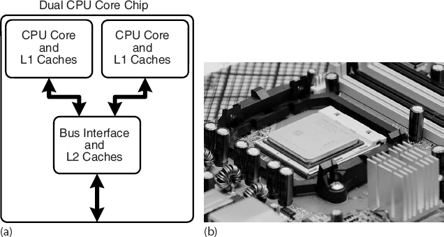
Figure 10.5 (a) A generic view of the Intel core-2 dual-core processor, with CPU-local level-1 caches and a shared, on-die level-2 cache (courtesy of D. Schmitz), (b) The AMD Athlon 64 X2 3600 dual-core CPU (Wikimedia Commons).

10.6 CPU Design: Vector Processors

Often the most demanding part of a scientific computation involves matrix operations. On a classic (von Neumann) scalar computer, the addition of two vectors of physical length 99 to form a third, ultimately requires 99 sequential additions (Table 10.2). There is actually much behind-the-scenes work here. For each element i there is the fetch of a(i) from its location in memory, the fetch of b(i) from its location in memory, the addition of the numerical values of these two elements in a CPU register, and the storage in memory of the sum in c(i). This fetching uses up time and is wasteful in the sense that the computer is being told again and again to do the same thing.

When we speak of a computer doing vector processing, we mean that there are hardware components that perform mathematical operations on entire rows or columns of matrices as opposed to individual elements. (This hardware can also handle single-subscripted matrices, that is, mathematical vectors.) In the vector processing of [A] + [B] = [C], the successive fetching of and addition of the elements A and B are grouped together and overlaid, and Z 64–256 elements (the section size) are processed with one command, as seen in Table 10.3. Depending on the array size, this method may speedup the processing of vectors by a factor of approximately 10. If all Z elements were truly processed in the same step, then the speedup would be ~ 64-256.

Vector processing probably had its heyday during the time when computer manufacturers produced large mainframe computers designed for the scientific and military communities. These computers had proprietary hardware and software and were often so expensive that only corporate or military laboratories could afford them. While the Unix and then PC revolutions have nearly eliminated these large vector machines, some do exist, as well as PCs that use vector processing in their video cards. Who is to say what the future holds in store?

Table 10.2 Computation of matrix [C] = [A] + [B]-

Step 1	Step 2	…	Step 99
c(1) = a(1) + b(1)	c(2) = a(2) + b(2)	…	c(99) = a(99) + b(99)

Table 10.3 Vector processing of matrix [A] + [B] = [C].

Step 1	Step 2	…	Step Z
c(1) = a(1) + b(1)
	c(2) = a(2) + b(2)
		…
			c(Z) = a(Z) + b(Z)

10.7 Introduction to Parallel Computing

There is a little question that advances in the hardware for parallel computing are impressive. Unfortunately, the software that accompanies the hardware often seems stuck in the 1960s. In our view, message passing and GPU programming have too many details for application scientists to worry about and (unfortunately) requires coding at an elementary level reminiscent of the early days of computing. However, the increasing occurrence of clusters in which the nodes are symmetric multiprocessors has led to the development of sophisticated compilers that follow simpler programming models; for example, partitioned global address space compilers such as CoArray Fortran, Unified Parallel C, and Titanium. In these approaches, the programmer views a global array of data and then manipulates these data as if they were contiguous. Of course, the data really are distributed, but the software takes care of that outside the programmer’s view. Although such a program may make use of processors less efficiently than would a hand-coded program, it is a lot easier than redesigning your program. Whether it is worth your time to make a program more efficient depends on the problem at hand, the number of times the program will be run, and the resources available for the task. In any case, if each node of the computer has a number of processors with a shared memory and there are a number of nodes, then some type of a hybrid programming model will be needed.

10.8 Parallel Semantics (Theory)

We saw earlier that many of the tasks undertaken by a high-performance computer are run in parallel by making use of internal structures such as pipelined and segmented CPUs, hierarchical memory, and separate I/O processors. While these tasks are run “in parallel,” the modern use of parallel computing or parallelism denotes applying multiple processors to a single problem (Quinn, 2004). It is a computing environment in which some number of CPUs are running asynchronously and communicating with each other in order to exchange intermediate results and coordinate their activities.

For an instance, consider the matrix multiplication:

[10.4]

Mathematically, this equation makes no sense unless [A] equals the identity matrix [I]. However, it does make sense as an algorithm that produces new value of B on the LHS in terms of old values of B on the RHS:

[10.5]

[10.6]

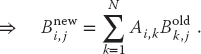
Because the computation of for specific values of i and j is independent of all other values of and can be computed in parallel, or each row or column of [B^new] can be computed in parallel. If B were not a matrix, then we could just calculate B = AB with no further ado. However, if we try to perform the calculation using just matrix elements of [B] by replacing the old values with the new values as they are computed, then we must somehow establish that the B_k,j on the RHS of (10.6) are the values of [B] that existed before the matrix multiplication.

This is an example of data dependency, in which the data elements used in the computation depend on the order in which they are used. A way to account for this dependency is to use a temporary matrix for [B^new], and then to assign [B] to the temporary matrix after all multiplications are complete:

[10.7]

[10.8]

In contrast, the matrix multiplication [C] = [A][B] is a data parallel operation in which the data can be used in any order. So already we see the importance of communication, synchronization, and understanding of the mathematics behind an algorithm for parallel computation.

The processors in a parallel computer are placed at the nodes of a communication network. Each node may contain one CPU or a small number of CPUs, and the communication network may be internal to or external to the computer. One way of categorizing parallel computers is by the approach they utilize in handling instructions and data. From this viewpoint there are three types of machines:

Single instruction, single data (SISD) These are the classic (von Neumann) serial computers executing a single instruction on a single data stream before the next instruction and next data stream are encountered.

Single instruction, multiple data (SIMD) Here instructions are processed from a single stream, but the instructions act concurrently on multiple data elements. Generally, the nodes are simple and relatively slow but are large in number.

Multiple instructions, multiple data (MIMD) In this category, each processor runs independently of the others with independent instructions and data. These are the types of machines that utilize message-passing packages, such as MPI, to communicate among processors. They may be a collection of PCs linked via a network, or more integrated machines with thousands of processors on internal boards, such as the Blue Gene computer described in Section 10.15. These computers, which do not have a shared memory space, are also called multicomputers. Although these types of computers are some of the most difficult to program, their low cost and effectiveness for certain classes of problems have led to their being the dominant type of parallel computer at present.

The running of independent programs on a parallel computer is similar to the multitasking feature used by Unix and PCs. In multitasking (Figure 10.4a), several independent programs reside in the computer’s memory simultaneously and share the processing time in a round robin or priority order. On a SISD computer, only one program runs at a single time, but if other programs are in memory, then it does not take long to switch to them. In multiprocessing (Figure 10.4b), these jobs may all run at the same time, either in different parts of memory or in the memory of different computers. Clearly, multiprocessing becomes complicated if separate processors are operating on different parts of the same program because then synchronization and load balance (keeping all the processors equally busy) are concerns.

In addition to instructions and data streams, another way of categorizing parallel computation is by granularity. A grain is defined as a measure of the computational work to be performed, more specifically, the ratio of computation work to communication work.

Coarse-grain parallel Separate programs running on separate computer systems with the systems coupled via a conventional communication network. An illustration is six Linux PCs sharing the same files across a network but with a different central memory system for each PC. Each computer can be operating on a different, independent part of one problem at the same time.

Medium-grain parallel Several processors executing (possibly different) programs simultaneously while accessing a common memory. The processors are usually placed on a common bus (communication channel) and communicate with each other through the memory system. Medium-grain programs have different, independent, parallel subroutines running on different processors. Because the compilers are seldom smart enough to figure out which parts of the program to run where, the user must include the multitasking routines in the program.¹⁾

Fine-grain parallel As the granularity decreases and the number of nodes increases, there is an increased requirement for fast communication among the nodes. For this reason, fine-grain systems tend to be custom-designed machines. The communication may be via a central bus or via shared memory for a small number of nodes, or through some form of high-speed network for massively parallel machines. In the latter case, the user typically divides the work via certain coding constructs, and the compiler just compiles the program. The program then runs concurrently on a user-specified number of nodes. For example, different for loops of a program may be run on different nodes.

10.9 Distributed Memory Programming

An approach to concurrent processing that, because it is built from commodity PCs, has gained dominant acceptance for coarse- and medium-grain systems is distributed memory. In it, each processor has its own memory and the processors exchange data among themselves through a high-speed switch and network. The data exchanged or passed among processors have encoded to and from addresses and are called messages. The clusters of PCs or workstations that constitute a Beowulf²⁾ are examples of distributed memory computers (Figure 10.6). The unifying characteristic of a cluster is the integration of highly replicated compute and communication components into a single system, with each node still able to operate independently. In a Beowulf cluster, the components are commodity ones designed for a general market, as are the communication network and its high-speed switch (special interconnects are used by major commercial manufacturers, but they do not come cheaply). Note: A group of computers connected by a network may also be called a cluster, but unless they are designed for parallel processing, with the same type of processor used repeatedly and with only a limited number of processors (the front end) onto which users may log in, they are not usually called a Beowulf.

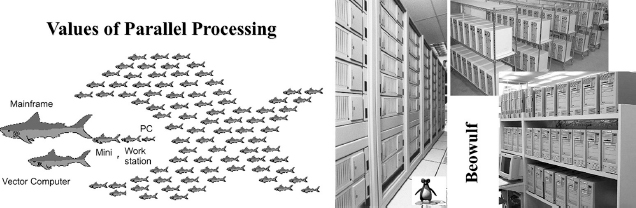
Figure 10.6 Two views of parallel computing (courtesy of Yuefan Deng).

The literature contains frequent arguments concerning the differences among clusters, commodity clusters, Beowulfs, constellations, massively parallel systems, and so forth (Dongarra et al., 2005). Although, we recognize that there are major differences between the clusters on the top 500 list of computers and the ones that a university researcher may set up in his or her lab, we will not distinguish these fine points in the introductory materials we present here.

For a message-passing program to be successful, the data must be divided among nodes so that, at least for a while, each node has all the data it needs to run an independent subtask. When a program begins execution, data are sent to all the nodes. When all the nodes have completed their subtasks, they exchange data again in order for each node to have a complete new set of data to perform the next subtask. This repeated cycle of data exchange followed by processing continues until the full task is completed. Message-passing MIMD programs are also single-program, multiple-data programs, which means that the programmer writes a single program that is executed on all the nodes. Often a separate host program, which starts the programs on the nodes, reads the input files and organizes the output.

10.10 Parallel Performance

Imagine a cafeteria line in which all the servers appear to be working hard and fast yet the ketchup dispenser has some relish partially blocking its output and so everyone in line must wait for the ketchup lovers up front to ruin their food before moving on. This is an example of the slowest step in a complex process determining the overall rate. An analogous situation holds for parallel processing, where the ketchup dispenser may be a relatively small part of the program that can be executed only as a series of serial steps. Because the computation cannot advance until these serial steps are completed, this small part of the program may end up being the bottleneck of the program.

As we soon will demonstrate, the speedup of a program will not be significant unless you can get ~90% of it to run in parallel, and even then most of the speedup will probably be obtained with only a small number of processors. This means that you need to have a computationally intense problem to make parallelization worthwhile, and that is one of the reasons why some proponents of parallel computers with thousands of processors suggest that you should not apply the new machines to old problems but rather look for new problems that are both big enough and well-suited for massively parallel processing to make the effort worthwhile.

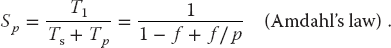
The equation describing the effect on speedup of the balance between serial and parallel parts of a program is known as Amdahl’s law (Amdahl, 1967; Quinn, 2004). Let

[10.9]

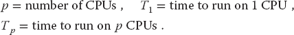
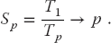
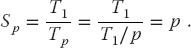
The maximum speedup S_p attainable with parallel processing is thus

[10.10]

In practice, this limit is never met for a number of reasons: some of the program is serial, data and memory conflicts occur, communication and synchronization of the processors take time, and it is rare to attain a perfect load balance among all the processors. For the moment, we ignore these complications and concentrate on how the serial part of the code affects the speedup. Let f be the fraction of the program that potentially may run on multiple processors. The fraction 1 – f of the code that cannot be run in parallel must be run via serial processing and thus takes time:

[10.11]

The time T_p spent on the p parallel processors is related to T_s by

[10.12]

That being so, the maximum speedup as a function of f and the number of processors is

[10.13]

Some theoretical speedups are shown in Figure 10.7 for different numbers of processors p. Clearly the speedup will not be significant enough to be worth the trouble unless most of the code is run in parallel (this is where the 90% of the in-parallel figure comes from). Even an infinite number of processors cannot increase the speed of running the serial parts of the code, and so it runs at one processor speed. In practice, this means many problems are limited to a small number of processors, and that only 10–20% of the computer’s peak performance is often all that is obtained for realistic applications.

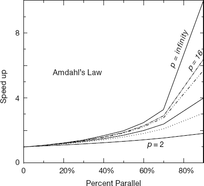
Figure 10.7 The theoretical maximum speedup of a program as a function of the fraction of the program that potentially may be run in parallel. The different curves correspond to different numbers of processors.

10.10.1 Communication Overhead

As discouraging as Amdahl’s law may seem, it actually overestimates speedup because it ignores the overhead for parallel computation. Here we look at communication overhead. Assume a completely parallel code so that its speedup is

[10.14]

The denominator is based on the assumption that it takes no time for the processors to communicate. However, in reality it takes a finite time, called latency, to get data out of memory and into the cache or onto the communication network. In addition, a communication channel also has a finite bandwidth, that is, a maximum rate at which data can be transferred, and this too will increase the communication time as large amounts of data are transferred. When we include communication time T_c, the speedup decreases to

[10.15]

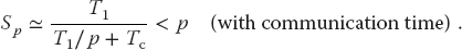
For the speedup to be unaffected by communication time, we need to have

[10.16]

This means that as you keep increasing the number of processors p, at some point the time spent on computation T₁/p must equal the time T_c needed for communication, and adding more processors leads to greater execution time as the processors wait around more to communicate. This is another limit, then, on the maximum number of processors that may be used on any one problem, as well as on the effectiveness of increasing processor speed without a commensurate increase in communication speed.

The continual and dramatic increase in the number of processors being used in computations is leading to a changing view as to how to judge the speed of an algorithm. Specifically, the slowest step in a process is usually the rate-determining step, yet with the increasing availability of CPU power, the slowest step is more often the access to or communication among processors. Such being the case, while the number of computational steps is still important for determining an algorithm’s speed, the number and amount of memory access and interprocessor communication must also be mixed into the formula. This is currently an active area of research in algorithm development.

10.11 Parallelization Strategies

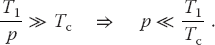
A typical organization of a program containing both serial and parallel tasks is given in Table 10.4. The user organizes the work into units called tasks, with each task assigning work (threads) to a processor. The main task controls the overall execution as well as the subtasks that run independent parts of the program (called parallel subroutines, slaves, guests, or subtasks). These parallel subroutines can be distinctive subprograms, multiple copies of the same subprogram, or even Python for loops.

It is the programmer’s responsibility to establish that the breakup of a code into parallel subroutines is mathematically and scientifically valid and is an equivalent formulation of the original program. As a case in point, if the most intensive part of a program is the evaluation of a large Hamiltonian matrix, you may want to evaluate each row on a different processor. Consequently, the key to parallel programming is to identify the parts of the program that may benefit from parallel execution. To do that the programmer should understand the program’s data structures (discussed soon), know in what order the steps in the computation must be performed, and know how to coordinate the results generated by different processors.

The programmer helps speedup the execution by keeping many processors simultaneously busy and by avoiding storage conflicts among different parallel subprograms. You do this load balancing by dividing your program into subtasks of approximately equal numerical intensity that will run simultaneously on different processors. The rule of thumb is to make the task with the largest granularity (workload) dominant by forcing it to execute first and to keep all the processors busy by having the number of tasks an integer multiple of the number of processors. This is not always possible.

Table 10.4 A typical organization of a program containing both serial and parallel tasks.

The individual parallel threads can have shared or local data. The shared data may be used by all the machines, while the local data are private to only one thread. To avoid storage conflicts, design your program so that parallel subtasks use data that are independent of the data in the main task and in other parallel tasks. This means that these data should not be modified or even examined by different tasks simultaneously. In organizing these multiple tasks, reduce communication overhead costs by limiting communication and synchronization. These costs tend to be high for fine-grain programming where much coordination is necessary. However, do not eliminate communications that are necessary to ensure the scientific or mathematical validity of the results; bad science can do harm!

10.12 Practical Aspects of MIMD Message Passing

It makes sense to run only the most numerically intensive codes on parallel machines. Frequently, these are very large programs assembled over a number of years or decades by a number of people. It should come as no surprise, then, that the programming languages for parallel machines are primarily Fortran, which now has explicit structures for the compiler to parallelize, and 0 C. (In the past, we have not obtained good speedup with Java and MPI, yet FastMPJ and MPJ Express have fixed the problems.)

Effective parallel programming becomes more challenging as the number of processors increases. Computer scientists suggest that it is best not to attempt to modify a serial code but instead rewrite one from scratch using algorithms and subroutine libraries best suited to parallel architecture. However, this may involve months or years of work, and surveys find that ~70% of computational scientists revise existing codes instead (Pancake, 1996).

Most parallel computations at present are performed on multiple instruction, multiple-data computers via message passing using MPI. Next we outline some practical concerns based on user experience (Dongarra et al., 2005; Pancake, 1996).

Parallelism carries a price tag There is a steep learning curve requiring intensive effort. Failures may occur for a variety of reasons, especially because parallel environments tend to change often and get “locked up” by a programming error. In addition, with multiple computers and multiple operating systems involved, the familiar techniques for debugging may not be effective.

Preconditions for parallelism If your program is run thousands of times between changes, with execution time in days, and you must significantly increase the resolution of the output or study more complex systems, then parallelism is worth considering. Otherwise, and to the extent of the difference, parallelizing a code may not be worth the time investment.

The problem affects parallelism You must analyze your problem in terms of how and when data are used, how much computation is required for each use, and the type of problem architecture.

Perfectly parallel This is when the same application is run simultaneously on different data sets, with the calculation for each data set independent (e.g., running multiple versions of a Monte Carlo simulation, each with different seeds, or analyzing data from independent detectors). In this case, it would be straightforward to parallelize with a respectable performance to be expected.

Fully synchronous The same operation applied in parallel to multiple parts of the same data set, with some waiting necessary (e.g., determining positions and velocities of particles simultaneously in a molecular dynamics simulation). Significant effort is required, and unless you balance the computational intensity, the speedup may not be worth the effort.

Loosely synchronous Different processors do small pieces of the computation but with intermittent data sharing (e.g., diffusion of groundwater from one location to another). In this case, it would be difficult to parallelize and probably not worth the effort.

Pipeline parallel Data from earlier steps processed by later steps, with some overlapping of processing possible (e.g., processing data into images and then into animations). Much work may be involved, and unless you balance the computational intensity, the speedup may not be worth the effort.

10.12.1 High-Level View of Message Passing

Although it is true that parallel computing programs may become very complicated, the basic ideas are quite simple. All you need is a regular programming language like Python, C, or Fortran, plus four communication statements:³⁾

• send: One processor sends a message to the network.
• receive: One processor receives a message from the network.
• myid: An integer that uniquely identifies each processor.
• numnodes: An integer giving the total number of nodes in the system.

Once you have made the decision to run your program on a computer cluster, you will have to learn the specifics of a message-passing system such as MPI. Here we give a broader view. When you write a message-passing program, you intersperse calls to the message-passing library with your regular Python, Fortran, or C program. The basic steps are as follows:

1. Submit your job from the command line or a job control system.
2. Have your job start additional processes.
3. Have these processes exchange data and coordinate their activities.
4. Collect these data and have the processes stop themselves.

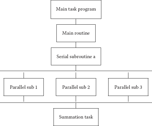
Figure 10.8 A master process and two slave processes passing messages. Notice how in this not-well-designed program there are more sends than receives, and consequently the results may depend upon the order of execution, or the program may even lock up.

We show this graphically in Figure 10.8 where at the top we see a master process create two slave processes and then assign work for them to do (arrows). The processes then communicate with each other via message passing, output their data to files, and finally terminate.

What can go wrong Figure 10.8 also illustrates some of the difficulties:

• The programmer is responsible for getting the processes to cooperate and for dividing the work correctly.
• The programmer is responsible for ensuring that the processes have the correct data to process and that the data are distributed equitably.
• The commands are at a lower level than those of a compiled language, and this introduces more details for you to worry about.
• Because multiple computers and multiple operating systems are involved, the user may not receive or understand the error messages produced.
• It is possible for messages to be sent or received not in the planned order.
• A race condition may occur in which the program results depend upon the specific ordering of messages. There is no guarantee that slave 1 will get its work performed before slave 2, even though slave 1 may have started working earlier (Figure 10.8).
• Note in Figure 10.8 how different processors must wait for signals from other processors; this is clearly a waste of time and has potential for deadlock.
• Processes may deadlock, that is, wait for a message that never arrives.

10.12.2 Message Passing Example and Exercise

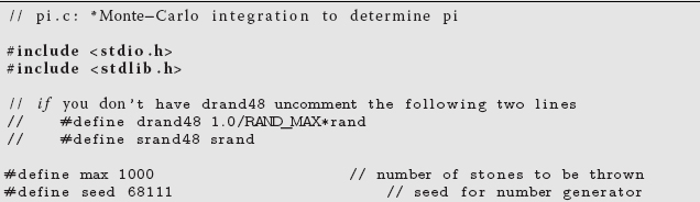
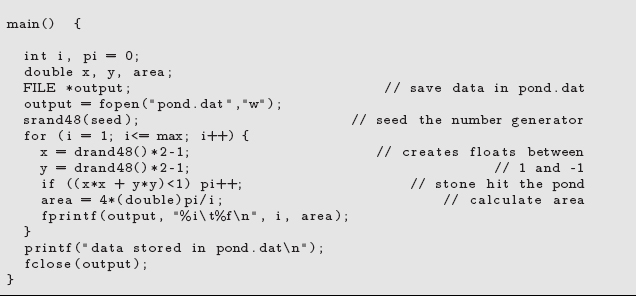
Start with a simple serial program you have already written that is a good candidate for parallelization. Specifically, one that steps through parameter space in order to generate its results is a good candidate because you can have parallel tasks working on different regions of parameter space. Alternatively, a Monte Carlo calculation that repeats the same step many times is also a good candidate because you can run copies of the program on different processors, and then add up the results at the end. For example, Listing 10.1 is a serial calculation of π by Monte Carlo integration in the C language:

Listing 10.1 Serial calculation of π by Monte Carlo integration.

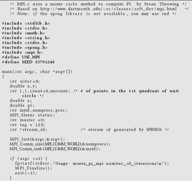
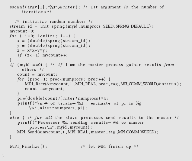
Modify your serial program so that different processors are used and perform independently, and then have all their results combined. For example, Listing 10.2 is a parallel version of pi.c that uses the message passing interface (MPI). You may want to concentrate on the arithmetic commands and not the MPI ones at this point.

Listing 10.2 MPI.c: Parallel calculation of π by Monte Carlo integration using MPI.

Although this small a problem is not worth your efforts in order to obtain a shorter run time, it is worth investing your time to gain some experience in parallel computing.

10.13 Scalability

A common discussion at HPC and Supercomputing conferences of the past heard application scientists get up, after hearing about the latest machine with what seemed like an incredible number of processors, and ask “But how can I use such a machine on my problem, which takes hours to run, but is not trivially parallel like your example?” The response from the computer scientist was often something like “You just need to think up some new problems that are more appropriate to the machines being built. Why use a supercomputer for a problem you can solve on a modern laptop?” It seems that these anecdotal exchanges have now been incorporated into the fabric of parallel computing under the title of scalability. In the most general sense, scalability is defined as the ability to handle more work as the size of the computer or application grows.

As we have already indicated, the primary challenge of parallel computing is deciding how best to break up a problem into individual pieces that can each be computed separately. In an ideal world, a problem would scale in a linear fashion, that is, the program would speedup by a factor of N when it runs on a machine having N nodes. (Of course, as N → ∞ the proportionality cannot hold because communication time must at some point dominate). In present day terminology, this type of scaling is called strong scaling, and refers to a situation in which the problem size remains fixed while the number of number of nodes (the machine scale) increases. Clearly then, the goal when solving a problem that scales strongly is to decrease the amount of time it takes to solve the problem by using a more powerful computer. These are typically CPU-bound problems and are the hardest ones to yield something close to a linear speedup.

In contrast to strong scaling in which the problem size remains fixed, in weak scaling we have applications of the type our CS colleagues referred to earlier; namely, ones in which we make the problem bigger and bigger as the number of processors increases. So here, we would have linear or perfect scaling if we could increase the size of the problem solved in proportion to the number N of nodes.

To illustrate the difference between strong and weak scaling, consider Figure 10.9 (based on a lecture by Thomas Sterling). We see that for an application that scales perfectly strongly, the work carried out on each node decreases as the scale of the machine increases, which of course means that the time it takes to complete the problem decreases linearly. In contrast, we see that for an application that scales perfectly weakly, the work carried out by each node remains the same as the scale of the machine increases, which means that we are solving progressively larger problems in the same time as it takes to solve smaller ones on a smaller machine.

The concepts of weak and strong scaling are ideals that tend not to be achieved in practice, with real world applications being a mix of the two. Furthermore, it is the combination of application and computer architecture that determines the type of scaling that occurs. For example, shared memory systems and distributed-memory, message passing systems scale differently. Furthermore, a data parallel application (one in which each node can work on its own separate data set) will by its very nature scale weakly.

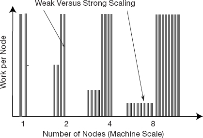
Figure 10.9 A graphical representation of weak vs. strong scaling. Weak scaling keeps each node doing the same amount of work as the problem is made bigger. Strong scaling has each node doing less work (running for less time) as the number of nodes is made bigger.

Before we go on and set you working on some examples of scaling, we should introduce a note of caution. Realistic applications tend to have various levels of complexity and so it may not be obvious just how to measure the increase in “size” of a problem. As an instance, it is known that the solution of a set of N linear equations via Gaussian elimination requires floating-point operations (flops). This means that doubling the number of equations does not make the “problem” twice as large, but rather eight times as large! Likewise, if we are solving partial differential equations on a 3D spatial grid and a 1D time grid, then the problem size would scale like N⁴. In this case, doubling the problem size would mean increasing N by only 2^1/4 1.19.

10.13.1 Scalability Exercises

We have given above, and included in the Codes directory, a serial code pi.c that computes π/4 by Monte Carlo integration of a quarter of a unit circle. We have also given the code MPIpi.c that computes π by the same algorithm using MPI to compute the algorithm in parallel. Your exercise is to see how well this application scales. You can modify the codes we have given, or you can write your own.

1. Determine the CPU time required to calculate π with the serial calculation using 1000 iterations (stone throws). Make sure that this is the actual run time and does not include any system time. (You can get this type of information, depending upon the operating system, by inserting timer calls in your program.)
2. Get the MPI code running for the same number (1000) of iterations.
3. First do some running that constitutes a strong scaling test. This means keeping the problem size constant, or in other words, keeping N_iter = 1000. Start by running the MPI code with only one processor doing the numerical computation. A comparison of this to the serial calculation gives you some idea of the overhead associated with MPI.
4. Again keeping N_iter = 1000, run the MPI code for 2, 4, 8, and 16 computing nodes. In any case, make sure to go up to enough nodes so that the system no longer scales. Record the run time for each number of nodes.
5. Make a plot of run time vs. number of nodes from the data you have collected.
6. Strong scalability here would yield a straight line graph. Comment on your results.
7. Now do some running that constitutes a weak scaling test. This means increasing the problem size simultaneously with the number of nodes being used. In the present case, increasing the number of iterations, N_iter.
8. Run the MPI code for 2, 4, 8, and 16 computing nodes, with proportionally larger values for N_iter in each case (2000, 4000, 8000, 16 000, etc.). In any case, make sure to go up to enough nodes so that the system no longer scales.
9. Record the run time for each number of nodes and make a plot of the run time vs. number of computing nodes.
10. Weak scaling would imply that the run time remains constant as the problem size and the number of compute nodes increase in proportion. Comment on your results.
11. Is this problem more appropriate for weak or strong scaling?

10.14 Data Parallelism and Domain Decomposition

As you have probably realized by this point, there are two basic, but quite different, approaches to creating a program that runs in parallel. In task parallelism, you decompose your program by tasks, with differing tasks assigned to different processors, and with great care taken to maintain load balance, that is, to keep all processors equally busy. Clearly you must understand the internal workings of your program in order to do this, and you must also have made an accurate profile of your program so that you know how much time is being spent in various parts.

In data parallelism, you decompose your program based on the data being created or acted upon, with differing data spaces (domains) assigned to different processors. In data parallelism, there often must be data shared at the boundaries of the data spaces, and therefore synchronization among the data spaces. Data parallelism is the most common approach and is well suited to message-passing machines in which each node has its own private data space, although this may lead to a large amount of data transfer at times.

When planning how to decompose global data into subspaces suitable for parallel processing, it is important to divide the data into contiguous blocks in order to minimize the time spent on moving data through the different stages of memory (page faults). Some compilers and operating systems help you in this regard by exploiting spatial locality, that is, by assuming that if you are using a data element at one location in data space, then it is likely that you may use some nearby ones as well, and so they too are made readily available. Some compilers and operating systems also exploit temporal locality, that is, by assuming that if you are using a data element at one time, then there is an increased probability that you may use it again in the near future, and so it too is kept handy. You can help optimize your programs by taking advantage of these localities while programming.

As an example of domain decomposition, consider the solution of a partial differential equation by a finite difference method. It is known from classical electrodynamics that the electric potential U(x) in a charge-free region of 2D space satisfies Laplace’s equation (fully discussed in Section 19.4):

[10.17]

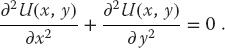
We see that the potential depends simultaneously on x and y, which is what makes it a partial differential equation. The electric charges, which are the source of the field, enter indirectly by specifying the potential values on some boundaries or charged objects.

As shown in Figure 10.10, we look for a solution on a lattice (x, y) values separated by finite difference Δ in each dimension and specified by discrete locations on the lattice:

[10.18]

When the finite difference expressions for the derivatives are substituted into (10.17), and the equation is rearranged, we obtain the finite-difference algorithm for the solution of Laplace’s equation:

[10.19]

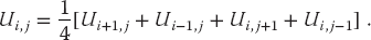
This equation says that when we have a proper solution, it will be the average of the potential at the four nearest neighbors (Figure 10.10). As an algorithm, (10.19) does not provide a direct solution to Laplace’s equation but rather must be repeated many times to converge upon the solution. We start with an initial guess for the potential, improve it by sweeping through all space, taking the average over nearest neighbors at each node, and keep repeating the process until the solution no longer changes to some level of precision or until failure is evident. When converged, the initial guess is said to have relaxed into the solution.

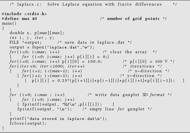
In Listing 10.3, we have a serial code laplace.c that solves the Laplace equation in two dimensions for a straight wire kept at 100 V in a grounded box, using the relaxation algorithm (10.19). There are five basic elements of the code:

1. Initialize the potential values on the lattice.
2. Provide an initial guess for the potential, in this case U = 0 except for the wire at 100 V.
3. Maintain the boundary values and the source term values of the potential at all times.
4. Iterate the solution until convergence ((10.19) being satisfied to some level of precision) is obtained.
5. Output the potential in a form appropriate for 3D plotting.

As you can see, the code is a simple pedagogical example with its essential structure being the array p[40][40] representing a (small) regular lattice. Industrial strength applications might use much larger lattices as well as adaptive meshes and hierarchical multigrid techniques.

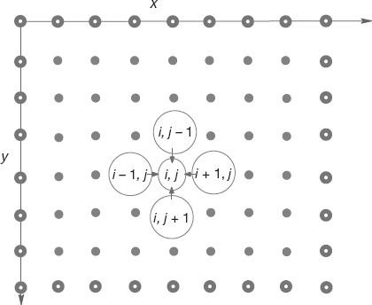
Figure 10.10 A representation of the lattice in a 2D rectangular space upon which Laplace’s equation is solved using a finite difference approach. The lattice sites with white centers correspond to the boundary of the physical system, upon which boundary conditions must be imposed for a unique solution. The large circles in the middle of the lattice represent the algorithm used to solve Laplace’s equation in which the potential at the point (x, y) = (i, j)Δ is set to the average of the potential values at the four nearest-neighbor points.

When thinking of parallelizing this program, we note an algorithm being applied to a space of data points, in which case we can divide the domain into sub-spaces and assign each subspace to a different processor. This is domain decomposition or data parallelism. In essence, we have divided a large boundary-value problem into an equivalent set of smaller boundary-value problems that eventually get fit back together. Often extra storage is allocated on each processor to hold the data values that get communicated from neighboring processors. These storage locations are referred to as ghost cells, ghost rows, ghost columns, halo cells, or overlap areas.

Two points are essential in domain decomposition: (i) Load balancing is critical, and is obtained here by having each domain contain the same number of lattice points. (ii) Communication among the processors should be minimized because this is a slow process. Clearly the processors must communicate to agree on the potential values at the domain boundaries, except for those boundaries on the edge of the box that remain grounded at 0 V. But because there are many more lattice sites that need computing than there are boundaries, communication should not slow down the computation severely for large lattices.

To see an example of how this is carried out, the serial code poisson_1d.c solves Laplace’s equation in 1D, and poisson_parallel_ld.c solves the same 1D equation in parallel (codes courtesy of Michel Vallieres). This code uses an accelerated version of the iteration algorithm using the parameter Ω, a separate method for domain decomposition, as well as ghost cells to communicate the boundaries.

Listing 10.3 laplace.c Serial solution of Laplace’s equation using a finite difference technique.

10.14.1 Domain Decomposition Exercises

1. Get the serial version of either laplace.c or laplace.f running.
2. Increase the lattice size to 1000 and determine the CPU time required for convergence to six places. Make sure that this is the actual run time and does not include any system time. (You can get this type of information, depending upon the operating system, by inserting timer calls in your program.)
3. Decompose the domain into four subdomains and get an MPI version of the code running on four compute nodes. [Recall, we give an example of how to do this in the Codes directory with the serial code poisson_1d.c and its MPI implementation, poisson_parallel_1d.c (courtesy of Michel Vallières).]
4. Convert the serial code to three dimensions. This makes the application more realistic, but also more complicated. Describe the changes you have had to make.
5. Decompose the 3D domain into four subdomains and get an MPI version of the code running on four compute nodes. This can be quite a bit more complicated than the 2D problem.
6. Conduct a weak scaling test for the 2D or 3D code.
7. Conduct a strong scaling test for the 2D or 3D code.

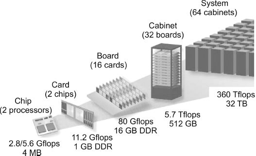
Figure 10.11 The building blocks of Blue Gene (from Gara et al. (2005)).

10.15 Example: The IBM Blue Gene Supercomputers

Whatever figures we give to describe the latest supercomputer will be obsolete by the time you read them. Nevertheless, for the sake of completeness, and to set the present scale, we do it anyway. At the time of this writing, one of the fastest computers is the IBM Blue Gene/Q member of the Blue Gene series. In its largest version, its 96 racks contains 98 304 compute nodes with 1.6 million processor cores and 1.6 PB of memory (Gara et al., 2005). In June 2012, it reached a peak speed of 20.1 PFLOPS.

The name Blue Gene reflects the computer’s origin in gene research, although Blue Genes are now general-purpose supercomputers. In many ways, these are computers built by committee, with compromises made in order to balance cost, cooling, computing speed, use of existing technologies, communication speed, and so forth. As a case in point, the compute chip has 18 cores, with 16 for computing, 1 for assisting the operating system with communication, and 1 as a redundant spare in case one of the others was damaged. Having communication on the chip reflects the importance of communication for distributed-memory computing (there are both on- and off-chip distributed memories). And while the CPU is fast with 204.8 GFLOPS at 1.6 GHz, there are faster ones made, but they would generate so much heat that it would not be possible to obtain the extreme scalability up to 98 304 compute nodes. So with the high-efficiency figure of 2.1 GFLOPS/watt, Blue Gene is considered a “green” computer.

We look more closely now at one of the original Blue Genes, for which we were able to obtain illuminating figures (Gara et al., 2005). Consider the building-block view in Figure 10.11. We see multiple cores on a chip, multiple chips on a card, multiple cards on a board, multiple boards in a cabinet, and multiple cabinets in an installation. Each processor runs a Linux operating system (imagine what the cost in both time and money would be for Windows!) and utilizes the hardware by running a distributed memory MPI with C, C++, and Fortran90 compilers.

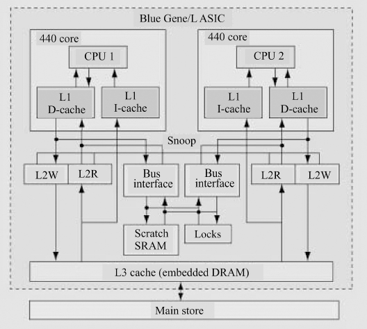
Figure 10.12 The single-node memory system (as presented by Gara et al. (2005)).

Blue Gene has three separate communication networks (Figure 10.13). At the heart of the network is a 3D torus that connects all the nodes, for example, Figure 10.13 a shows a sample torus of 2 × 2 × 2 nodes. The links are made by special link chips that also compute; they provide both direct neighbor–neighbor communications and cut-through communication across the network. The result of this sophisticated communications network is that there are approximately the same effective bandwidth and latencies (response times) between all nodes. However, the bandwidth may be affected by interference among messages, with the actual latency also depending on the number of hops to get from one node to another.⁴⁾ A rate of 1.4Gb/s is obtained for node-to-node communication. The collective network in Figure 10.13b is used for collective communications among processors, such as a broadcast. Finally, the control and gigabit ethernet network (Figure 10.13c) is used for I/O to communicate with the switch (the hardware communication center) and with ethernet devices.

The computing heart of Blue Gene is its integrated circuit and the associated memory system (Figure 10.12). This is essentially an entire computer system on a chip, with the exact specifications depending upon the model, and changing with time.

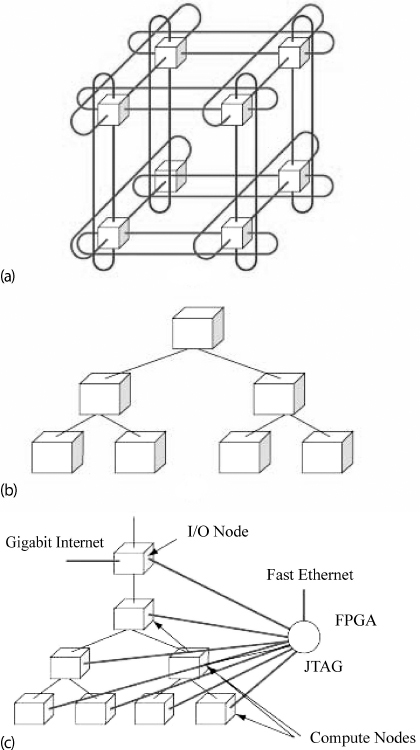
Figure 10.13 (a) A 3D torus connecting 2 × 2 × 2 compute nodes. (b) The global collective memory system. (c) The control and Gb-ethernet memory system (from Gara et al. (2005)).

10.16 Exascale Computing via Multinode-Multicore GPUs

The current architecture of top-end supercomputers (Figure 10.14) uses a very large numbers of nodes, with each node containing a chip set that includes multiple cores as well as a graphical processing unit (GPU) attached to the chip set⁵⁾. In the near future, we expect to see laptop computers capable of teraflops (10¹² floating-point operations per second), deskside computers capable of petaflops, and supercomputers at the exascale, in terms of both flops and memory, probably with millions of nodes.

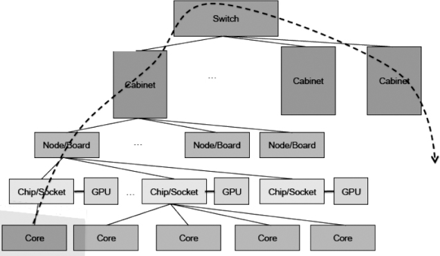
Figure 10.14 A schematic of an exascale computer in which, in addition to each chip having multiple cores, a graphical processing unit is attached to each chip (adapted from Dongarra (2011)).

Look again at the schematic in Figure 10.14. As in Blue Gene, there really are large numbers of chip boards and large numbers of cabinets. Here we show just one node and one cabinet and not the full number of cores. The dashed line in Figure 10.14 represents communications, and it is seen to permeate all components of the computer. Indeed, communications have become such an essential part of modern supercomputers, which may contain 100s of 1000s of CPUs, that the network interface “card” may be directly on the chip board. Because a computer of this sort contains shared memory at the node level and distributed memory at the cabinet or higher levels, programming for the requisite data transfer among the multiple elements is a fundamental challenge, with significant new investments likely to occur (Dongarra et al., 2014).

1) Some experts define our medium grain as coarse grain yet this distinction changes with time.

2) Presumably there is an analogy between the heroic exploits of the son of Ecgtheow and the nephew of Hygelac in the 1000 C.E. poem Beowulf and the adventures of us common folk assembling parallel computers from common elements that have surpassed the performance of major corporations and their proprietary, multimillion-dollar supercomputers.

3) Personal communication, Yuefan Deng.

4) The number of hops is the number of devices a given data packet passes through.

5) GPUs and their programming are discussed in Chapter 11.